G Exercise 05
Last updated: 2026-02-12 16:04:46
G.2 Question 1
- Recreate the DEM of the Carmel area in UTM, as shown in the right panel in Figure 9.10, using the following code section:
library(stars)
dem1 = read_stars('data/srtm_43_06.tif')
dem2 = read_stars('data/srtm_44_06.tif')
pol = st_read('data/israel_borders.shp', quiet = TRUE)
dem = st_mosaic(dem1, dem2)
dem = dem[, 5687:6287, 2348:2948]
names(dem) = 'elevation'
dem = st_warp(src = dem, crs = 32636, method = 'near', cellsize = 90)- Calculate a point geometry of the peak of the Carmel mountain, by finding the centroid of the pixel that has the highest elevation in the image.
- Calculate the nearest point in the Mediterranean sea from the peak, assuming the sea area is all of the
NApixels in the image. (Hint: calculate the distances from the peak to allNApixels, converted to points, then usewhich.minto find the nearest one.) - Plot the DEM, the peak, the nearest “sea” point, the line connecting them, and the distance, as shown in Figure G.1.
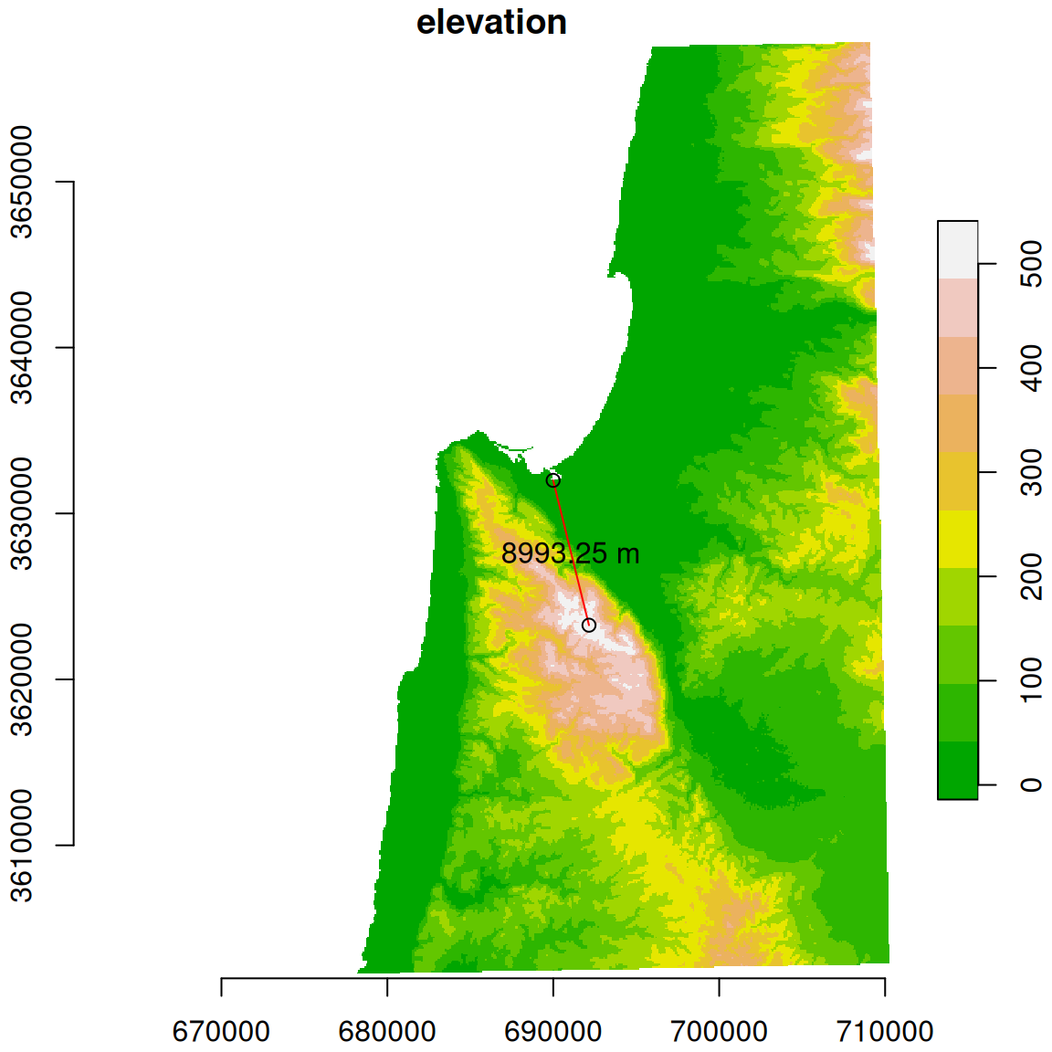
Figure G.1: Length of the shortest line between Carmel mountain peak and the Mediterranean sea
(50 points)
G.3 Question 2
- Read the
'MOD13A3_2000_2019.tif'raster, with monthly NDVI values, into astarsobject namedr, then reproject it to UTM withst_warp(r,crs=32636).
- Use
'MOD13A3_2000_2019_dates.csv'to assign date values to raster bands (see Section 6.3.2). - Read the Shapefile named
'nafot.shp', which includes polygons of “Nafa” administrative regions in Israel, and reproject it to UTM as well. - Calculate the average NDVI for each polygon in each date.
- Plot the resulting time series of average NDVI for each of the “Nafot”, as shown in Figure G.2. Hint: you can start from an empty plot using
plot(..., col=NA), then add the NDVI times series usinglinesinforloop; see Section 6.1.3. - Mark the time series of “Nafa” where the lowest average NDVI was observed, during the studied period, in red. The other “Nafa” should be displayed in grey. Don’t use “Nafa” indices or names, or any other specific values; instead calculate the required indices in your code.
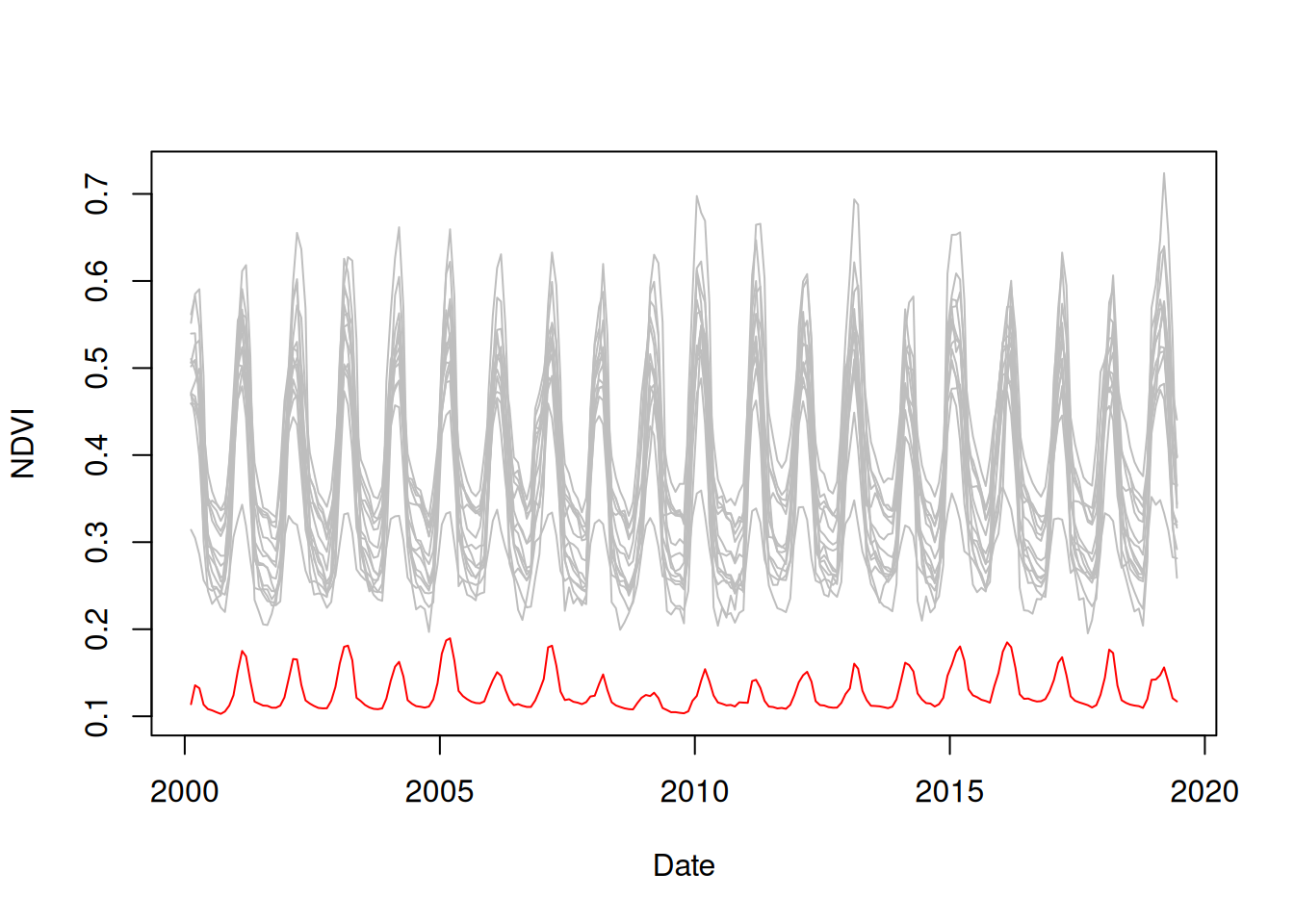
Figure G.2: Average NDVI over time in “Nafa” polygons, the “Nafa” with the lowest observed average NDVI is marked in red
(50 points)
G.4 Question 3
- Read the
'MOD13A3_2000_2019.tif'raster, with monthly NDVI values, into astarsobject namedr, then reproject it to UTM withst_warp(r,crs=32636) - Read
'MOD13A3_2000_2019_dates.csv'to get the dates corresponding to raster bands (see Section 6.3.2) - Read the Shapefile named
'nafot.shp', which includes polygons of “Nafa” administrative regions in Israel, and reproject it to UTM as well - Calculate the date when NDVI was lowest, for each “Nafa”. That is, the date when the average NDVI of all Nafa pixels was lower than on any other date.
- Print a table with the results (Nafa names and their calculated dates), sorted from earliest to latest date
##           nafa       date
## 2    Jerusalem 2000-09-15
## 13 Be'er Sheva 2000-09-15
## 15    Tel Aviv 2001-09-15
## 1        Zefat 2001-10-15
## 4     Yizre'el 2001-10-15
## 5         Akko 2001-10-15
## 6        Golan 2001-10-15
## 9       Sharon 2002-10-15
## 10       Ramla 2002-10-15
## 14 Petah Tiqwa 2002-10-15
## 8       Hadera 2008-09-15
## 7        Haifa 2010-10-15
## 11     Rehovot 2010-10-15
## 12    Ashqelon 2010-10-15
## 3     Kinneret 2017-09-15