Chapter 2 Vectors
Last updated: 2026-02-12 15:59:58
Aims
Our aims in this chapter are:
- Learn how to work with R code files
- Get to know the simplest data structure in R, the vector
- Learn about subsetting, one of the fundamental operations with data
2.1 R code files
2.1.1 What are code files
In Chapter 1, we typed short and simple expressions into the R console. As we progress, however, the code we write will get longer and more complex. To be able to edit and save longer code, the code is kept in code files. Thus there are two “methods” for executing R code:
- Typing the code in the console and pressing Enter
- Sending code stored in a code file to the console (we will see how, in a moment)
Either way, the code is interpreted, and we get the results or outputs (Figure 2.1).
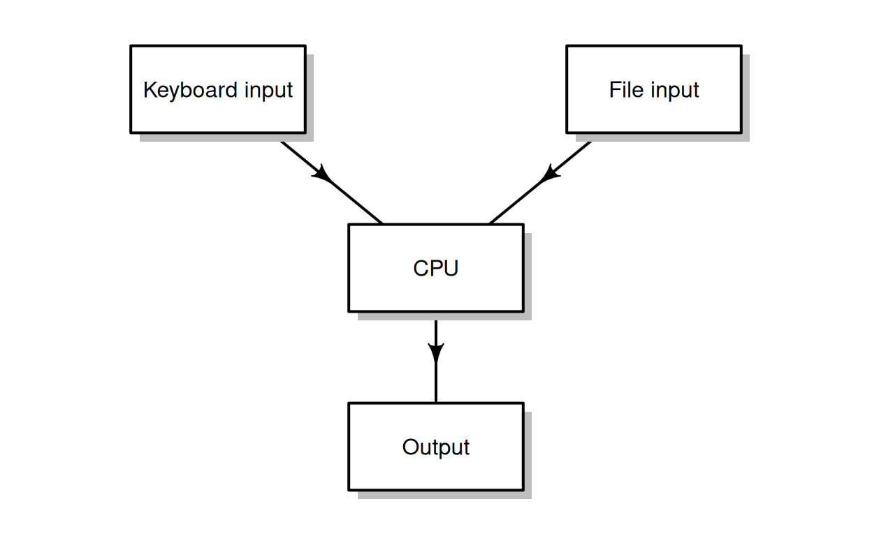
Figure 2.1: Methods of executing R code: sending code from a code file, or typing code using the keyboard
2.1.2 Working with plain text
Computer code is stored in code files as plain text. When writing computer code, we must use a plain text editor, such as Notepad++ or RStudio (Section 1.2). A word processor, such as Microsoft Word, is not a good choice for writing code, because:
- Documents created with a word processor contain elements other than plain text (such as highlighting, font types, sizes, colors, etc.), which are therefore ignored by the interpreter, leading to confusion
- Word processors can automatically correct “mistakes” thereby introducing unintended changes in our code, such as capitalizing:
max(1)→Max(1)
Any plain text file can be used to store R code, though, conventionally, R code files have the .R file extension.
2.1.3 Code files in RStudio
To start working with a code file in RStudio, we can do one of the following:
- Create a new code file, selecting File → New File… → R Script from the menu (or pressing Ctrl+Shift+N)
- Open an existing code file, selecting File → Open File… from the menu (or pressing Ctrl+O)
The new file, or a modified existing file, can be saved by selecting File → Save from the menu (or pressing Ctrl+S).
Open the code file named
volcano.Rwhich is included in the book materials in RStudio.
There are several methods to execute code from a code file, by sending it to the console. The most obvious one is to copy a section of code, then paste it in the console, and press Enter, but this is not very convenient. Instead we usually do one of the following:
- We can send a single expression, by placing the cursor on a particular line and pressing Ctrl+Enter. The expression is executed and the cursor advances to the next line, which means we can press Ctrl+Enter again to execute it too, and so on.
- We can send a selection of several lines of code, by marking the section and pressing Ctrl+Enter.
- We can execute all lines from the top of the code file to the line where the cursor is, by pressing Ctrl+Alt+B.
For example, we can run the file volcano.R which draws a 3D image of a volcano (Figure 2.2). The file is contained in the book materials. See Appendix A for the link to download the files.

Figure 2.2: 3D image of the volcano dataset
Try each of the above three methods to execute R code with the
volcano.Rcode file. Running the entire code file, by selecting all code with Ctrl+A and pressing Ctrl+Enter, produces a 3D image of a volcano in the graphical output panel (Figure 2.2).
2.1.4 RStudio keyboard stortcuts
RStudio has numerous keyboard shortcuts for making it easier to edit and execute code files, some of which we already mentioned in the previous section. The most useful RStudio keyboard shortcuts are given in Table 2.1.
| Shortcut | Action |
|---|---|
| Ctrl+1 | Moving cursor to the code editor |
| Ctrl+2 | Moving cursor to the console |
| Ctrl+Enter | Running the current selection or line |
| Ctrl+Alt+B | Running from top to current line |
| Ctrl+Shift+C | Comment/uncomment |
| Tab | Auto-complete |
| Ctrl+D | Delete line |
| Ctrl+Shift+D | Duplicate line |
| Ctrl+F | Find and replace |
| Ctrl+S | Save |
2.2 Assignment
So far we have been using R by typing expressions into the command line and observing the result on screen. That way, R functions as a “calculator”; the results are not kept in computer memory (Figure 2.3).

Figure 2.3: Simple R expressions are evaluated and printed
Storing objects in the temporary computer memory (RAM) is called assignment. In an assignment expression, we are storing an object, under a certain name, in the RAM (Figure 2.4). Assignment is done using the assignment operator. Assignment is an essential operation in programming, because it makes automation possible—reaching the goal step by step, while storing intermediate products. An assignment expression consists of:
- The expression whose result we want to store
- The assignment operator,
=or<- - The name which will be assigned to the object
For example, the following expression assigns the result of the arithmetic calculation (6617747987-6617746521)/10 into a variable named rateEstimate:

Figure 2.4: An assignment expression stores an object in the RAM
When we type an object name in the console, R accesses an object stored under that name in the RAM, and calls the print function on the object (Figure 2.5):

Figure 2.5: Accessing an object stored in the RAM
What happens when we assign a new value to an existing object? The old value gets deleted, and the object is associated with a new value:
Note the difference between the == and = operators! = is an assignment operator:
while == is a conditional operator (Section 1.3.4) to test for equality:
Which user-defined objects are currently in memory? The ls function returns a character vector (see Section 2.3 below) with their names:
Why did we write
ls()and notls?
2.3 Vectors
2.3.1 What is a vector?
The vector is the simplest data structure in R, and the first data structure we learn about in this book. A vector, in R, is an ordered collection of values of the same type, such as:
- Numbers—
numeric(numbers with a decimal point), orinteger(whole numbers) - Text—
character - Logical—
logical
Recall that these are the same three types of “constant values” we saw in Chapter 1. In fact, R doesn’t have a special class for individual constant values. A constant value in R is actually represented by a vector of length 1.
The distinction between the numeric and integer classes (Section 1.3.11) is not very important for our purposes. Both of these two classes are used to represent numbers, and R automatically converts from one to another, as needed. We are mentioning both only because you may encounter either one when working with numbers. In this book, we will refer to both numeric and integer vectors as “numeric”, for convenience.
2.3.2 The c function
A vector of length 1 can be created simply by typing a value, such as 600 or "Hello", as we have already seen (Section 1.3). A vector of length >1 can be created in several ways. The most straightforward method is to use the c function, which combines its inputs—vectors of length 1, or more—into a new vector, in the specified order. For example:
Note that the c function is not restricted to combining individual values (i.e., vectors of length 1). It can be used to combine any number of vectors, of any length. For example, the following expression combines four vectors—of length 3, 1, 3 and 2—into a new vector of length 9:
Here is another example of using the c function, this time to combine four character values into a vector of length 4:
2.3.3 Vector subsetting (individual elements)
We can access individual vector elements using the [ operator and a numeric index. That way, we can get a subset with an individual vector element:
Note that numeric indices in R start at 1! This is unlike Python, C, JavaScript, and many other programming languages, where numeric indices start at 0.
Here is another example:
Note the three components of an expression for accessing a vector element:
- The vector being subsetted (
counts[4]) - Square brackets (
counts[4]) - The index (
counts[4])
We can also make an assignment into a vector subset, for example to replace an individual element:
In this example, we made an assignment into a subset with a single element. As we will see later on, we can assign values into a subset of any length, using the same method (Section 2.3.9).
2.3.4 Calling functions on a vector
There are numerous functions for calculating vector properties in R. The length, min, max, range, mean, and sum functions are most commonly used. Here is a demonstration of these functions:
In what way is the
rangefunction different from the other functions shown above?
Contrariwise, there are functions that operate on each vector element, separately, returning a vector of results having the same length as the input:
sqrt(x)  # Square root
## Warning in sqrt(x): NaNs produced
## [1] 1.000000 2.449490 1.732051      NaN 1.414214
Why does the output of
sqrt(x)containNaN?
Note that the last expression produced a warning. A warning, in R, signals to the user that something suspicious or notable has happened. A warning differs from an error (Section 1.3.7) in that when a warning is raised, the expression is executed nevertheless. Contrariwise, when an error is raised, code evaluation stops and the expression (and subsequent expressions, if any) is not executed by the interpreter.
2.3.5 The recycling rule (arithmetic)
Binary operations, such as arithmetic (Section 1.3.2) and conditional (Section 1.3.4) operators, when applied on two vectors, are done element-by-element. The result is, then, a vector of the respective results. For example, the following expression:
is interpreted as:
Here are three more examples, demonstrating the element-by-element behavior using other operators, *, >, and <:
What happens when the input vector lengths do not match? In such case, the shorter vector gets “recycled”. For example, when one of the vectors is of length 3 and the other vector is of length 6, then the shorter vector (of length 3) is replicated two times, until it matches the longer vector (Figure 2.6). Thus, the expression:
is equivalent to the expression:

Figure 2.6: Vector recycling
When one of the vectors is of length 1 and the other is of length 4, the shorter vector (of length 1) is replicated 4 times:
When one of the vectors is of length 2 and the other is of length 6, the shorter vector (of length 2) is replicated 3 times:
What happens when the longer vector length is not a multiple of the shorter vector length? In such case, recycling is “incomplete”, as indicated by a warning message. In the following example, the shorter vector is recycled “1.5 times”:
c(1, 2)    * c(1, 2, 3)
## Warning in c(1, 2) * c(1, 2, 3): longer object length is not a multiple of
## shorter object length
## [1] 1 4 3Incomplete recycling is rarely something we want to do in practice. Therefore, the latter warning is usually an indication that something is wrong in our code.
2.3.6 Consecutive and repetitive vectors
2.3.6.1 Introduction
Other than the c function (Section 2.3.2), there are three commonly used methods for creating consecutive or repetitive vectors:
2.3.6.2 Consecutive vectors
The : operator is used to create a vector of consecutive values in steps of 1:
or in steps of -1:
The seq function provides a more general way to create a consecutive vector with any step size, not necessarily 1 or -1. The three most useful parameters of the seq function are:
from—Where to startto—When to endby—Step size
For example:
The above examples of the seq function are also examples of passing more than one argument in a function call (Section 1.3.6). You may also have noticed that the arguments are named. We are going to elaborate on the syntax rules of using more than one argument, in a function call in R, in a moment (Section 2.3.7).
2.3.6.3 Repetitive vectors
The rep function replicates its argument to create a repetitive vector:
x—What to replicatetimes—How many times to replicate the entire vectoreach—How many times to replicate each element
For example, using times we can replicate the entire vector the specified number of times:
Alternatively, we can use each to replicate each element the specified number of times:
2.3.7 Function calls
Using the seq function, we will demonstrate three properties of function calls. First, we can omit parameter names as long as the arguments are passed in the default order. For example, the following two function calls are identical, because the default order of the (first three) seq function parameters is from, to, and by:
Second, we can use any argument order as long as parameter names are specified. The following three function calls are identical, even though argument order is not the same, since the arguments are named:
Third, we can omit parameters that have a default argument, specified as part of the function definition. For example, the by parameter of seq has a default value of 1:
The parameters of a particular function, their order, and their default values (if any), can be found in the help file of every function (Section 1.3.12):
2.3.8 Vector subsetting (general)
So far, we created vector subsets using a numeric index which consists of a single value (Section 2.3.3), as in:
We can also use a vector of length >1 as an index. For example, the following expression returns the first and second elements of x, since the index is the vector c(1,2) (which we create using the : operator) (Section 2.3.6.2):
Note that the vector of indices can consist of any combination of indices whatsoever. It does not have to be consecutive, and it can even include repetitions:
lettersis a built-in vector of English letters, i.e.,c('a','b','c',...). What will be the result ofletters[rep(2,3)]?
Here is another example (Figure 2.7):

Figure 2.7: Vector subsetting with a vector of indices (1:3)
And here is one more example where the index is not consecutive:
Note, again, the components of the subsetting expression:
- The vector being subsetted (
counts[c(1:3, 7:9)]) - Square brackets (
counts[c(1:3, 7:9)]) - The index (
counts[c(1:3, 7:9)])
For the next examples, let’s create a vector of all even numbers between 1 and 100:
x = seq(2, 100, 2)
x
##  [1]   2   4   6   8  10  12  14  16  18  20  22  24  26  28  30  32  34  36  38
## [20]  40  42  44  46  48  50  52  54  56  58  60  62  64  66  68  70  72  74  76
## [39]  78  80  82  84  86  88  90  92  94  96  98 100
Can you think of another way to create the above vector, using the
:and*operators?
What is the meaning of the numbers in square brackets when printing the vector?
How can we check how many elements does x have? Recall the length function (Section 2.3.4):
Using this knowledge, here are two expression that return the value of the last element in x:
Which of the last two expressions is preferable? Why?
Which index can we use to get back the entire vector? We can use an index that contains all of the vector element indices, starting from 1 and up to length(x):
x[1:length(x)]
##  [1]   2   4   6   8  10  12  14  16  18  20  22  24  26  28  30  32  34  36  38
## [20]  40  42  44  46  48  50  52  54  56  58  60  62  64  66  68  70  72  74  76
## [39]  78  80  82  84  86  88  90  92  94  96  98 100
What index can we use to get the entire vector except for the last two elements?
What index can we use to get a reversed vector?
Note that there is a built-in function named rev for reversing a vector:
rev(x)
##  [1] 100  98  96  94  92  90  88  86  84  82  80  78  76  74  72  70  68  66  64
## [20]  62  60  58  56  54  52  50  48  46  44  42  40  38  36  34  32  30  28  26
## [39]  24  22  20  18  16  14  12  10   8   6   4   2
Note that, when requesting elements beyond the vector length, we get NA (Not Available) values. For example:
2.3.9 The recycling rule (assignment)
Earlier, we saw how the recycling rule applies to arithmetic and conditional operators (Section 2.3.5). The rule also applies to assignment.
For example, here we assign a vector of length 1 (NA) into a subset of length 6 (c(1:3,7:9)). As a result, NA is replicated six times, to match the subset:
Here, c(NA,99) is replicated three times, also to match the subset of length 6:
2.3.10 Logical vectors
2.3.10.1 Creating logical vectors
The third common type of vectors, in addition to numeric and character vectors, are logical vectors. A logical vector is composed of logical values (Section 1.3.4), TRUE and FALSE (or NA). For example:
Usually, we will not be creating logical vectors manually, but through applying a conditional operator (Section 1.3.4) on a numeric or character vector. For example:
Note how the recycling rule applies to conditional operators in the above expression.
An important property of logical vectors is, that, when arithmetic operations are applied, the logical vector is automatically converted to a numeric one, where TRUE becomes 1 and FALSE becomes 0. For example:
What is the meaning of the values
4and0.4in the above example?
2.3.10.2 Subsetting with logical vectors
So far, we used a numeric vector of indices when subsetting a vector (Sections 2.3.3 and 2.3.8). A logical vector can also be used as an index for subsetting. When using a logical vector of indices, the subset contains those elements which are in the same positions as the TRUE elements in the index. This means that the logical vector of indices needs to match the length of the vector being subsetted. If this is not the case, the logical vector is recycled.
For example:
Here is another example, where the logical vector of indices is created from the same vector being subsetted:
In this example, the logical vector counts<3:
specifies whether to include each of the elements of counts in the resulting subset (Figure 2.8).
What does the expression
counts[counts<3]do, in plain language?

Figure 2.8: Subsetting with a logical vector
Here are some more examples of subsetting with a logical index:
What does the output
integer(0), which we got in the last expression, mean?
The next example is slightly more complex; we select the elements of z whose square is larger than 8:
Let’s go over this step-by-step. First, z^2 gives a vector of squared z values (2 is recycled):
Then, each of the squares is compared to 8 (8 is recycled):
Finally, the logical vector z^2>8 is used for subsetting z.
2.3.11 Missing values
The is.na function is used to detect missing (NA) values (Section 1.3.5) in a vector. The is.na function:
- accepts a vector, of any type, and
- returns a
logicalvector, withTRUEin place ofNAvalues andFALSEin place of non-NAvalues.
For example, suppose we have a vector x where some of the values are missing:
The is.na function can be used to detect which values are missing:
How can we use the above expression to subset the non-missing values of
x?
A common mistake is to use comparison with NA to detect missing values, instead of is.na, as in:
Can you explain the above result?
Many of the functions that summarize vector properties (Section 2.3.4), such as sum and mean, have a parameter called na.rm. The na.rm parameter is used to determine whether NA values are excluded from the calculation. The default is na.rm=FALSE, meaning that NA values are not excluded. For example:
Why do we get
NAin the first expression?
What do you think will be the result of
length(x),NAor7? Execute the expression to check your answer.
How can we replace the
NAvalues inxwith the mean of its non-NAvalues?
2.4 Additional useful functions
2.4.1 any and all
Sometimes we want to figure out whether a logical vector:
- contains at least one
TRUEvalue; or - is entirely composed of
TRUEvalues.
We can use the any and all functions, respectively, to do those things.
The any function returns TRUE if at least one of the input vector values is TRUE, otherwise it returns FALSE. For example, let’s take a numeric vector x:
The expression any(x > 5) returns TRUE, which means that the vector x > 5 contains at least one TRUE value, i.e., at least one element of x is greater than 5:
The expression any(x > 88) returns FALSE, which means that the vector x > 88 contains no TRUE values, i.e., none of the elements of x are greater than 88:
The all function returns TRUE if all of the input vector values are TRUE, otherwise it returns FALSE. For example, the expression all(x > 5) returns FALSE, which means that the vector x > 5 contains at least one FALSE value, i.e., not all elements of x are greater than 5:
The expression all(x > -1) returns TRUE, which means that x > -1 is composed entirely of TRUE values, i.e., all elements of x are greater than -1:
In a way, any and all are inverse:
anydetermines if the logical vector contains at least oneTRUEvaluealldetermines if the logical vector contains at least oneFALSEvalue
Which expression can we use to get
TRUEif vectorxcontains at least oneNAvalue, orFALSEif it does not?
2.4.2 which
The which function converts a logical vector to a numeric one, with the indices of TRUE values. That way, we can find out the index of values that satisfy a given condition. For example, considering the vector x:
the expression which(x > 2.3) returns the indices of TRUE elements in x > 2.3, i.e., the indices of x elements which are greater than 2.3:
2.4.3 which.min and which.max
Related to which (Section 2.4.2) are functions which.min and which.max. The latter two functions return the index of the (first!) minimal or maximal value in a vector, respectively. For example, considering the vector x:
using which.min we can find out that the minimal value of x is in the 5th position:
while using which.max we can find out that the maximal value of x is in the 2nd position:
What expression can we use to find all indices (
2,7) of the maximal value inx?
Keep in mind that which, which.min, and which.max ignore NA values. For example:
2.4.4 The order function
The order function returns ordered vector indices, based on the order of vector values. In other words, order gives the index of the smallest value, the index of the second smallest value, etc., up to the index of the largest value. For example, given the vector x:
order(x) returns the indices 1:length(x), ordered from smallest to largest value:
This result tells us that the 5th element of x is the smallest, the 6th is the second smallest, and so on.
We can also get the reverse order with decreasing=TRUE:
How can we get a sorted vector of elements from
x, as shown below, using theorderfunction?
## [1] 0 1 2 2 3 6 62.4.5 paste and paste0
The paste function is used to “paste” text values. Its sep parameter determines the separating character(s), with the default being sep=" " (a space). For example:
Non-character vectors are automatically converted to character before pasting:
The recycling rule applies in paste too:
paste("image", 1:5, ".tif", sep = "")
## [1] "image1.tif" "image2.tif" "image3.tif" "image4.tif" "image5.tif"
Finally, the paste0 function is a shortcut for paste with sep="":