Last updated: 2026-03-04 01:41:59Spatial data
Introduction
In this section, we go over the basics of working with spatial data in Python. The chapter is divided into three parts, according to the packages we introduce:
shapely—for working with vector geometeriesgeopandas—for working with vector layersrasterio—for working with rasters
Note
This chapter serves as a brief summary of one of the topics which are prerequisites of the main contents of the book (Prerequisites). Readers who are already familiar with the material, can either skip this chapter, or go over it for recollection and self-check, before going further. Readers who are new to the material, can use this chapter as a checklist of the topics they need to focus on when learning the prerequisites of the book.
Note
For a detailed introduction to the topics presented in this chapter, see the following chapters from the Introduction to Spatial Data Programming with Python book:
Packages
import matplotlib.pyplot as plt
import numpy as np
import pandas as pd
import shapely
import geopy
import pyproj
import geopandas as gpd
import rasterio
import rasterio.plot
import osmnx as ox
import net2
Vector geometries with shapely
What is shapely?
The shapely package (Gillies et al. 2007--) is a Python package for representing vector geometries and making calculations with them. The package follows the Simple Features standard, and internally uses the widely adopted open-source GEOS software. From the practical point of view, shapely defined data structures for the seven commonly used geometry types in spatial analysis (Table 4.1):
shapely
| Type | Description |
|---|---|
Point |
A single coordinate |
LineString |
One or more line segments |
Polygon |
An area that is enclosed by a linear ring |
MultiPoint |
A collection of one or more Points |
MultiLineString |
A collection of one or more LineStrings |
MultiPolygon |
A collection of one or more Polygons |
GeometryCollection |
Collection of one or more geometries that can be of different types |
Coordinates to points
Geometries can be constructed from coordinate sequences, using the corresponding method depending on the geometry type (Table 4.1). For example, the simplest construction operation is creating a Point geometry from one pair of x-y coordinates, using function shapely.Point:
pnt1 = shapely.Point(-2, 1)Note that the result is a shapely geometry object of type Point:
type(pnt1)shapely.geometry.point.PointPrinting the object draws a small image of the geometry (Figure 4.1):
pnt1
shapely geometry of type Point
Passing a shapely object to print displays the Well-Known Text (WKT) representation of the geometry:
print(pnt1)POINT (-2 1)The reverse, i.e., extracting the coordinates from a Point geometry object, can be done through the .x and .y properties:
pnt1.x-2.0pnt1.y1.0or the .coords property:
list(pnt1.coords)[0](-2.0, 1.0)Points to line
A LineString geometry (Table 4.1) can be created by passing a list of Point geometries to function shapely.LineString. To demonstrate, let’s create a second point object, named pnt2:
pnt2 = shapely.Point(0, 0)The list [pnt1,pnt2] can be passed to shapely.LineString:
line1 = shapely.LineString([pnt1, pnt2])The resulting LineString geometry named line1 is shown in Figure 4.2:
line1
shapely geometry of type LineString
WKT to shapely
A string (str) in the WKT format can be transformed to a shapely geometry using function shapely.from_wkt:
line1 = shapely.from_wkt('LINESTRING (-2 1, 0 0, 1 3, 3 1.5)')We can check and see that line1 is indeed a shapely geometry object:
type(line1)shapely.geometry.linestring.LineStringFigure 4.3 shows line1 graphically:
line1
shapely geometry created from WKT string
shapely to WKT
The opposite conversion, from a shapely geometry to str, can be done using function str:
str(line1)'LINESTRING (-2 1, 0 0, 1 3, 3 1.5)'Geocoding (geopy)
Geocoding is the operation of converting textual addresses to spatial coordinates. Typically, geocoding methods are calling online geocoding services, such as the open-source Nominatim API which is based on OpenStreetMap data.
The geopy package provides access to several popular geocoding services through Python. When using geopy with the Nominatim API, we first need to provide a unique application name (so that our usage is labeled on the server):
geolocator = geopy.geocoders.Nominatim(user_agent="networks course")
geolocator
<geopy.geocoders.nominatim.Nominatim at 0x76a340ce12b0>The resulting object can then be used for geocoding, as follows:
result = geolocator.geocode('Beer-Sheva, Israel')
result
Location(באר שבע, נפת באר שבע, מחוז הדרום, ישראל, (31.2457442, 34.7925181, 0.0))The result contains the coordinates in the .longitude and .latitude properties:
result.longitude, result.latitude(34.7925181, 31.2457442)These can be used to construct a 'Point' geometry, as follows:
pnt = shapely.Point(result.longitude, result.latitude)
print(pnt)
POINT (34.7925181 31.2457442)Geocoding (osmnx)
The osmnx package provides the ox.geocoder.geocode function for geocoding. The function accepts a string, and returns the (lat,lon) (!), if successful. For example:
coords = ox.geocoder.geocode('Beer-Sheva, Israel')
coords
(31.2457442, 34.7925181)The coordinates can then be converted to a 'Point' geometry. Note that the coordinates must to be reversed from (lat,lon) to (lon,lat)!
pnt = shapely.Point(coords[1], coords[0])
print(pnt)
POINT (34.7925181 31.2457442)Nearest point on line
Our first example of a geometric calculation with shapely is locating the nearest point on a line, given a line and point (which is not necessarily on the line). To demonstrate, let’s define another point named pnt3:
pnt3 = shapely.Point(-1.5, 0.3)Figure 4.4 shows the line1 and pnt3 together, by combining them into a GeometryCollection (What is shapely?) and printing it:
shapely.GeometryCollection([line1, pnt3])
LineString and a Point geometries
Locating the nearest point is done using function shapely.ops.nearest_points. The result n is a tuple of length two with the nearest points in the two input geometries, respectively:
n = shapely.ops.nearest_points(line1, pnt3)
n
(<POINT (-1.32 0.66)>, <POINT (-1.5 0.3)>)In this example, n[0] is the point on line1 which is nearest to pnt3, while n[1] is the point on pnt3 which is nearest to line1 (which is identical to pnt3). Figure 4.5 shows the result:
shapely.GeometryCollection([line1, n[0], n[1]])
LineString, a Point geometry, and the nearest point to it one the LineString
Splitting line by points
Another spatial calculation provided by shapely is splitting splitting one geometry by another, using function shapely.ops.split. One possible workflow is splitting a line into several by point(s). To do that, the point(s) must be exactly one the line. For example, using n[0] calculated above (Figure 4.5):
line1_s = shapely.ops.split(line1, n[0])line1_s is a GeometryCollection with the “parts” of the input line. In this case, the line was split into two parts:
print(line1_s)GEOMETRYCOLLECTION (LINESTRING (-2 1, -1.32 0.66), LINESTRING (-1.32 0.66, 0 0, 1 3, 3 1.5))The parts of a GeometryCollection can be extracted into separate geometry objects using .geoms combined with a numeric index:
print(line1_s.geoms[0])LINESTRING (-2 1, -1.32 0.66)print(line1_s.geoms[1])LINESTRING (-1.32 0.66, 0 0, 1 3, 3 1.5)Spatial relations (shapely)
shapely contains numerous functions to evaluate pairwise relations between individual geometries. The methods accepts a pair of geometries, and return True or False, indicating whether the queried relation exists or not. The most useful of those is .intersects, which identifies intersections.
For example, .intersects can be used to illustrate that n[0] is a point on line1, while n[1] is not (Figure 4.5):
line1.intersects(n[0])Trueline1.intersects(n[1])FalseReprojection (shapely)
The shapely package does not incorporate the concept of Coordinate Reference Systems (CRS), and geometries are not associated with a CRS. That is, shapely geometries are composed of coordinates in an arbitrary planar CRS. Using an additional package named pyproj, however, we are able to transform, or reproject, shapely geometries.
Let’s demonstrate with an example. Consider pnt defined above:
print(pnt)POINT (34.7925181 31.2457442)As far as the computer is concerned, the coordinates of pnt specify a position in an arbitrary plain. We, however, have prior knowledge that these coordinates are in fact degrees of longitude and latitude (Geocoding (osmnx)), that is in the geographic WGS84 CRS, i.e., EPSG:4326. Now, suppose that we want to transform the geometry pnt to a different CRS, say, to UTM Zone 36N, i.e., EPSG:32636. Using pyproj, we do this in two steps. First, we define a “transformer” object, where we specify the source and target CRS, using pyproj.Transformer.from_crs:
transformer = pyproj.Transformer.from_crs(4326, 32636, always_xy=True)We store the object in a variable, such as hereby named transformer. In the second step, we apply the shapely.transform function on the geometry we would like to transform, passing the .transform property of the transformer object, and interleaved=False (which fits the pyproj transformer format), as follows:
pnt_new = shapely.transform(pnt, transformer.transform, interleaved=False)
print(pnt_new)
POINT (670697.1924195166 3458222.402040339)The result pnt_new contains modified coordinates, referring to the same location on earth but in a different CRS.
Practice
- Transform
pnt_newback toEPSG:4326 - You should get the original coordinates we started with, i.e.,
(34.7925181, 31.2457442)
The transformer object can be reused, in cases when we need to transform multiple geometries using the same transformation. For example, suppose we have a list with three points in EPSG:4326, which we want to transform to Web Mercator (EPSG:3857):
points = [pnt1, pnt2, pnt3]
points
[<POINT (-2 1)>, <POINT (0 0)>, <POINT (-1.5 0.3)>]Using list comprehension (list comprehension), here is how we can get a new list with the results:
transformer = pyproj.Transformer.from_crs(4326, 3857, always_xy=True)
[shapely.transform(i, transformer.transform, interleaved=False) for i in points]
[<POINT (-222638.982 111325.143)>, <POINT (0 0)>, <POINT (-166979.236 33396)>]Note that the geopandas package provides a higher-level workflow for transforming multiple geometries as once, as shown in Reprojection (geopandas).
Vector layers with geopandas
What is geopandas?
The geopandas package (Bossche et al. 2023) provides data structures and functions to work with vector layers in Python. The two fundamantal data structures in geopandas are:
GeoSeries—Geometry column, i.e., a collection ofshapelygeometries, associated with a CRS definition (possiblyNone)GeoDataFrame—Vector layer, i.e., aDataFramewhere one of the columns is aGeoSeries
To understand the data structures in geopandas, we will create a vector layer from scratch. The workflow is as follows:
- create a
listofshapelygeometries (GeoSeries from scratch), - convert it to a
GeoSeries(GeoSeries from scratch), and - convert the
GeoSeries, plus additional (zero or more) non-geometry columns, to aGeoDataFrame(GeoDataFrame from scratch).
GeoSeries from scratch
First, let’s create a list of shapely geometries. As an example, we will create a list with three Point geometries, representing hospitals in southern Israel, through geocoding (Geocoding (osmnx)):
locations = ['Soroka', 'Yoseftal', 'Barzilai']
locations
['Soroka', 'Yoseftal', 'Barzilai']addresses = [i + ' Hospital, Israel' for i in locations]
addresses['Soroka Hospital, Israel',
'Yoseftal Hospital, Israel',
'Barzilai Hospital, Israel']pnt = [ox.geocoder.geocode(i) for i in addresses]
pnt[(31.2582113, 34.8009331), (29.5541675, 34.9405596), (31.663251, 34.562429)]Recall that the input to ox.geocoder.geocode is a string, and the output is a tuple of the form (lat,lon). For any further spatial analysis, the coordinates need to be reversed to (lon,lat) (Geocoding (osmnx)):
pnt = [(i[1], i[0]) for i in pnt]
pnt
[(34.8009331, 31.2582113), (34.9405596, 29.5541675), (34.562429, 31.663251)]The coordinates can now be converted to shapely point geometries:
pnt = [shapely.Point(i) for i in pnt]
pnt
[<POINT (34.801 31.258)>, <POINT (34.941 29.554)>, <POINT (34.562 31.663)>]Finally, we transform the coordinates from WGS84 (EPSG:4326) to UTM (EPSG:32636) (Reprojection (shapely)):
transformer = pyproj.Transformer.from_crs(4326, 32636, always_xy=True)
pnt = [shapely.transform(i, transformer.transform, interleaved=False) for i in pnt]
pnt
[<POINT (671476.111 3459617.482)>,
<POINT (688011.999 3270955.999)>,
<POINT (648124.907 3504170.926)>]Now we are ready to move on, and transform our data to geopandas data structures. Here is how we transform a list of shapely geometries to a geometry column GeoSeries. Note the second (optional) argument, where we specify the CRS of the geometries:
geom = gpd.GeoSeries(pnt, crs=32636)
geom
0 POINT (671476.111 3459617.482)
1 POINT (688011.999 3270955.999)
2 POINT (648124.907 3504170.926)
dtype: geometryGeoDataFrame from scratch
Finally, the geometry column can be converted to a vector layer GeoDataFrame. A vector layer is a tabular data structure, where one of the columns is a geometry column. Technically speaking, a GeoDataFrame is a special case of a DataFrame (DataFrame from scratch) where:
- One of the columns is a
GeoSeries - The other columns, if any, are
Series
There are several ways to create a GeoDataFrame. The following expression is suitable for the scenario where a GeoSeries is combined with a dict representing the other non-geometry columns:
hospitals = gpd.GeoDataFrame(data={'name': locations}, geometry=geom)
hospitals| name | geometry | |
|---|---|---|
| 0 | Soroka | POINT (671476.111 3459617.482) |
| 1 | Yoseftal | POINT (688011.999 3270955.999) |
| 2 | Barzilai | POINT (648124.907 3504170.926) |
The GeoSeries which is part of an existing GeoDataFrame can be extracted using the .geometry property:
hospitals.geometry0 POINT (671476.111 3459617.482)
1 POINT (688011.999 3270955.999)
2 POINT (648124.907 3504170.926)
Name: geometry, dtype: geometryGeocoding (geopandas)
A GeoDataFrame can also be created straight from a list of addresses, using gpd.tools.geocode. For example:
hospitals2 = gpd.tools.geocode(addresses)
hospitals2| geometry | address | |
|---|---|---|
| 0 | POINT (34.80093 31.25821) | בית חולים סורוקה, ארלוזורוב, 84... |
| 1 | POINT (34.94056 29.55417) | בית החולים יוספטל, יותם, 880462... |
| 2 | POINT (34.55685 31.66487) | בי״ח ברזילי/חיל הים, חיל הים, 7... |
To match the structure of the GeoDataFrame we created in the last example, let’s rearrange the columns:
hospitals2['name'] = locations
hospitals2 = hospitals2[['name', 'geometry']]
hospitals2| name | geometry | |
|---|---|---|
| 0 | Soroka | POINT (34.80093 31.25821) |
| 1 | Yoseftal | POINT (34.94056 29.55417) |
| 2 | Barzilai | POINT (34.55685 31.66487) |
GeoSeries to list
Sometimes we need to transform a GeoSeries “back” to a list of shapely geometries. For example, this is useful when we want to apply a shapely function on each of the geometries inside a loop. A GeoSeries can be transformed to a list using the .to_list method, same as an “ordinary” Series (Series to list). For example:
geom.to_list()[<POINT (671476.111 3459617.482)>,
<POINT (688011.999 3270955.999)>,
<POINT (648124.907 3504170.926)>]or:
hospitals.geometry.to_list()[<POINT (671476.111 3459617.482)>,
<POINT (688011.999 3270955.999)>,
<POINT (648124.907 3504170.926)>]Writing vector layers
A GeoDataFrame can be exported to a file using the .to_file method. The .to_file method automatically detects the output format according to the file extension. For example, here is how we can export the hospitals layer into a GeoPackage file named hospitals.gpkg placed in the output directory:
hospitals.to_file('output/hospitals.gpkg')Vector layer from file
A GeoDataFrame can be imported from an existing vector layer file using the gpd.read_file function. For example, here we import a line layer of roads in Beer-Sheva from the file beer-sheva_edges.gpkg:
roads = gpd.read_file('output/beer-sheva_edges.gpkg')
roads| source | target | speed_kph | length | time | name | geometry | |
|---|---|---|---|---|---|---|---|
| 0 | 127675195 | 1775804621 | 63.12500 | 33.318135 | 1.900123 | שדרות בנ"צ כרמל | LINESTRING (673879.22 3459570.1... |
| 1 | 127675195 | 599614127 | 90.00000 | 14.697048 | 0.587882 | LINESTRING (673879.22 3459570.1... | |
| 2 | 280105509 | 946001975 | 60.00000 | 12.583977 | 0.755039 | שדרות יצחק רגר | LINESTRING (671254.039 3458787.... |
| ... | ... | ... | ... | ... | ... | ... | ... |
| 10341 | 12178896415 | 3920321928 | 50.00000 | 25.875941 | 1.863068 | LINESTRING (666778.531 3457441.... | |
| 10342 | 12178896415 | 3920326865 | 50.00000 | 340.343871 | 24.504759 | LINESTRING (666778.531 3457441.... | |
| 10343 | 12349570201 | 2619404125 | 48.37535 | 52.082648 | 3.875890 | ישמעאל | LINESTRING (671268.225 3456952.... |
10344 rows × 7 columns
here we import a point layer of gas stations in Beer-Sheva from the file named gas-stations.geojson:
stations = gpd.read_file('data/gas-stations.geojson')
stations| ADDRESS | Name | firma | lon | lat | geometry | |
|---|---|---|---|---|---|---|
| 0 | דרך מצדה באר שבע | מצדה | סונול | 34.770416 | 31.252988 | POINT (34.77042 31.25299) |
| 1 | דרך מצדה 226 | נאות מדבר | פז | 34.770640 | 31.253616 | POINT (34.77064 31.25362) |
| 2 | שד' דוד טוביהו 100 | טוביהו | דלק+סד''ש | 34.780509 | 31.246409 | POINT (34.78051 31.24641) |
| ... | ... | ... | ... | ... | ... | ... |
| 36 | אילן רמון | אילן רמון | דלק | 34.757597 | 31.256367 | POINT (34.7576 31.25637) |
| 37 | כיכר רוטשילד יחיל | בהקמה | בהקמה | 34.802752 | 31.243555 | POINT (34.80275 31.24356) |
| 38 | יהודה הנחתום 4 | 34.813940 | 31.257265 | POINT (34.81394 31.25726) |
39 rows × 6 columns
and here we import a polygonal layer of European countries from the europe.gpkg file:
europe = gpd.read_file('data/europe.gpkg')
europe| name | geometry | |
|---|---|---|
| 0 | Albania | POLYGON ((5250878.03 2039389.75... |
| 1 | Austria | POLYGON ((4839987.968 2803428.6... |
| 2 | Belarus | POLYGON ((5436932.506 3816251.1... |
| ... | ... | ... |
| 36 | Ukraine | POLYGON ((5788113.051 3443307.2... |
| 37 | United Kingdom | MULTIPOLYGON (((3455660.833 344... |
| 38 | Russia | MULTIPOLYGON (((7174520.945 329... |
39 rows × 2 columns
Reprojection (geopandas)
In spatial analysis involving more than one layer, we must make sure that all layers are in the same CRS. For example, inspecting the .crs property of the roads and stations layers reveals that they are in different CRS. Namely, roads is in EPSG:32636 (UTM, a projected CRS):
roads.crs<Projected CRS: EPSG:32636>
Name: WGS 84 / UTM zone 36N
Axis Info [cartesian]:
- E[east]: Easting (metre)
- N[north]: Northing (metre)
Area of Use:
- name: Between 30°E and 36°E, northern hemisphere between equator and 84°N, onshore and offshore. Belarus. Cyprus. Egypt. Ethiopia. Finland. Israel. Jordan. Kenya. Lebanon. Moldova. Norway. Russian Federation. Saudi Arabia. Sudan. Syria. Türkiye (Turkey). Uganda. Ukraine.
- bounds: (30.0, 0.0, 36.0, 84.0)
Coordinate Operation:
- name: UTM zone 36N
- method: Transverse Mercator
Datum: World Geodetic System 1984 ensemble
- Ellipsoid: WGS 84
- Prime Meridian: Greenwichstations, however, is in EPSG:4326 (WGS84, a geographic CRS):
stations.crs<Geographic 2D CRS: EPSG:4326>
Name: WGS 84
Axis Info [ellipsoidal]:
- Lat[north]: Geodetic latitude (degree)
- Lon[east]: Geodetic longitude (degree)
Area of Use:
- name: World.
- bounds: (-180.0, -90.0, 180.0, 90.0)
Datum: World Geodetic System 1984 ensemble
- Ellipsoid: WGS 84
- Prime Meridian: GreenwichThe .to_crs method is used to transform a GeoSeries or GeoDataFrame from one CRS to another. For example, here is how we can transform the stations layer to the same CRS as roads (EPSG:32636):
stations = stations.to_crs(roads.crs) # equivalent to: stations.to_crs(32636)
stations| ADDRESS | Name | firma | lon | lat | geometry | |
|---|---|---|---|---|---|---|
| 0 | דרך מצדה באר שבע | מצדה | סונול | 34.770416 | 31.252988 | POINT (668579.295 3458991.433) |
| 1 | דרך מצדה 226 | נאות מדבר | פז | 34.770640 | 31.253616 | POINT (668599.512 3459061.391) |
| 2 | שד' דוד טוביהו 100 | טוביהו | דלק+סד''ש | 34.780509 | 31.246409 | POINT (669552.25 3458277.577) |
| ... | ... | ... | ... | ... | ... | ... |
| 36 | אילן רמון | אילן רמון | דלק | 34.757597 | 31.256367 | POINT (667352.514 3459346.49) |
| 37 | כיכר רוטשילד יחיל | בהקמה | בהקמה | 34.802752 | 31.243555 | POINT (671675.848 3457995.631) |
| 38 | יהודה הנחתום 4 | 34.813940 | 31.257265 | POINT (672716.472 3459532.817) |
39 rows × 6 columns
Plotting (geopandas)
The .plot method can be used to draw an image of a GeoSeries or a GeoDataFrame. For example, Figure 4.6 shows the roads layer:
roads.plot();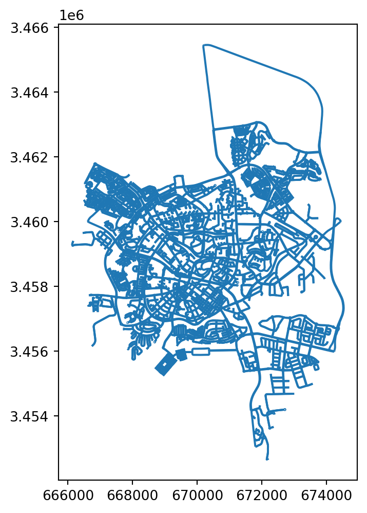
roads layer
Figure 4.7 demonstrates the use of the color and linewidth parameters of .plot:
roads.plot(color='grey', linewidth=0.5);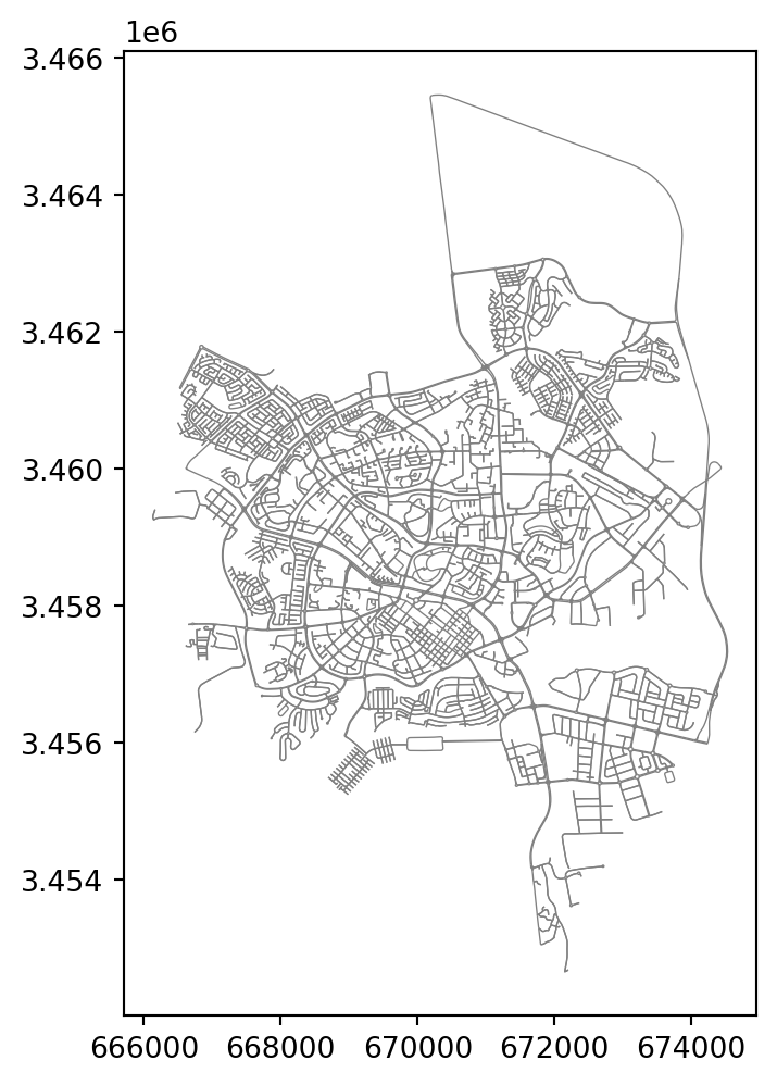
color and linewidth parameters of .plot
Figure 4.8 plots the stations layer:
stations.plot();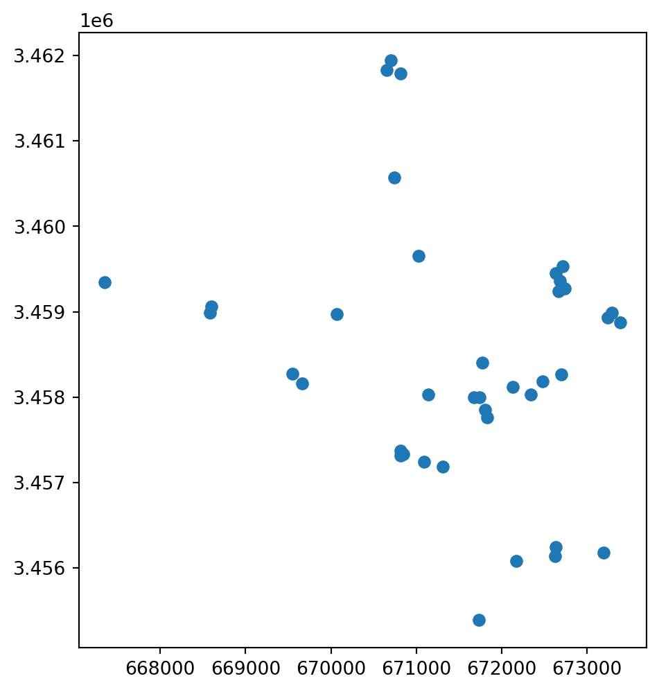
stations layer
Figure 4.9 demonstrates how two layers—roads and stations—can be displayed in one plot:
base = roads.plot(zorder=0)
stations.plot(ax=base, color='red', zorder=1);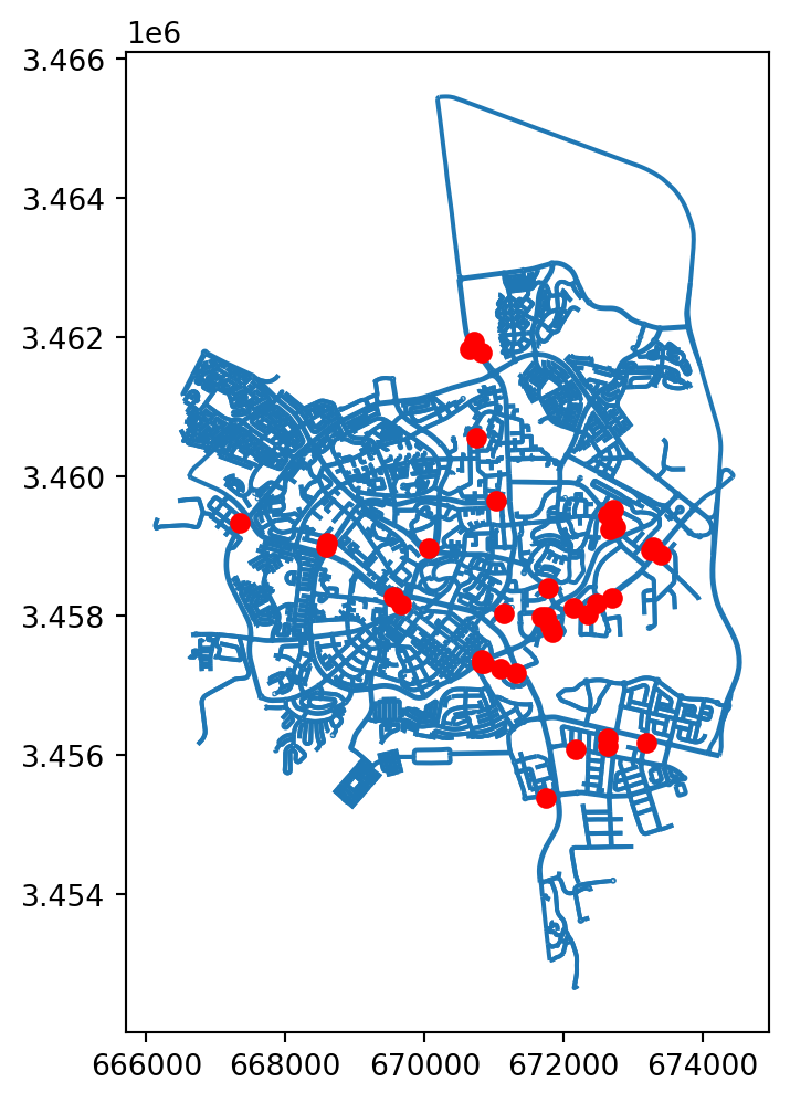
roads and stations—displayed in one plot
To add text labels on a map, we can use the .annotate method. In this case the plot needs to be initialized using plt.subplots. Then, spatial layers and annotations can be added to the same plot object to be displayed together. For example, Figure 4.10 shows two layers (roads and a subset of hospitals), and a text annotation with the hospital name. First let’s create a subset with the hospital of interest:
soroka = hospitals[hospitals['name'] == 'Soroka']
soroka| name | geometry | |
|---|---|---|
| 0 | Soroka | POINT (671476.111 3459617.482) |
Then, we can create the plot:
fig, ax = plt.subplots()
roads.plot(ax=ax, color='lightgrey', linewidth=0.5)
soroka.plot(ax=ax)
ax.annotate('Soroka', soroka.geometry.iloc[0].coords[0]);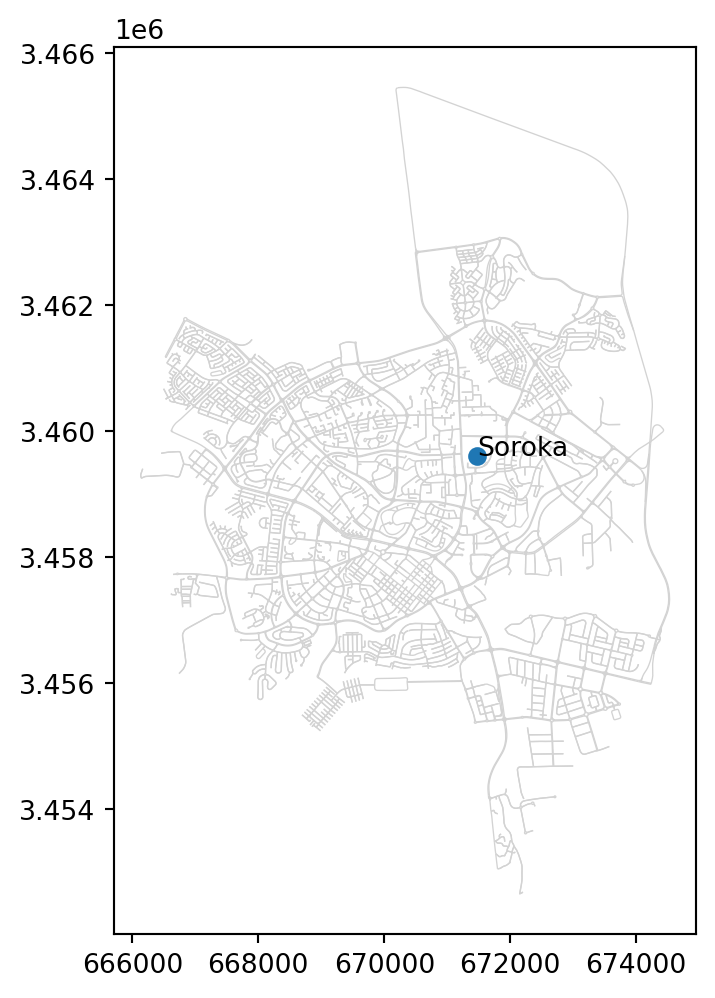
roads layer, the Soroka hospital from the hospitals layer, and a textual annotation “Soroka”
Note that .annotate expects a list or tuple of coordinates, which we extracted from the GeoDataFrame named soroka, as follows:
soroka.geometry.iloc[0].coords[0](671476.1105918102, 3459617.4824850867)Random points
In Exercise 08-02, you will be asked to create points in random locations within a given rectangular extent. Let’s see how this can be done. First, let’s define the extent according to the europe layer, using the .total_bounds property:
bounds = europe.total_bounds
bounds
array([2633231.15339975, 1448184.01014483, 7380192.43377843,
6394565.81286753])Now let’s “unpack” (Assignment) the coordinates into four separate variables:
xmin, ymin, xmax, ymax = boundsHere is how we can create 300 random points within the specified extent:
points = []
while len(points) < 300:
    random_point = shapely.Point([
        np.random.uniform(xmin, xmax),
        np.random.uniform(ymin, ymax)
    ])
    points.append(random_point)
When the loop ends, points is a list with 300 shapely geometries. Let’s convert it to a GeoSeries:
points = gpd.GeoSeries(points)
points
0 POINT (3107887.25 2449559.743)
1 POINT (5860876.824 4983831.575)
2 POINT (5983179.32 5350218.745)
...
297 POINT (5092421.242 6272156.32)
298 POINT (6674727.976 1929077.72)
299 POINT (4241056.183 3739125.418)
Length: 300, dtype: geometryFigure 4.11 shows the result:
base = europe.plot(color='none', edgecolor='grey')
points.plot(ax=base);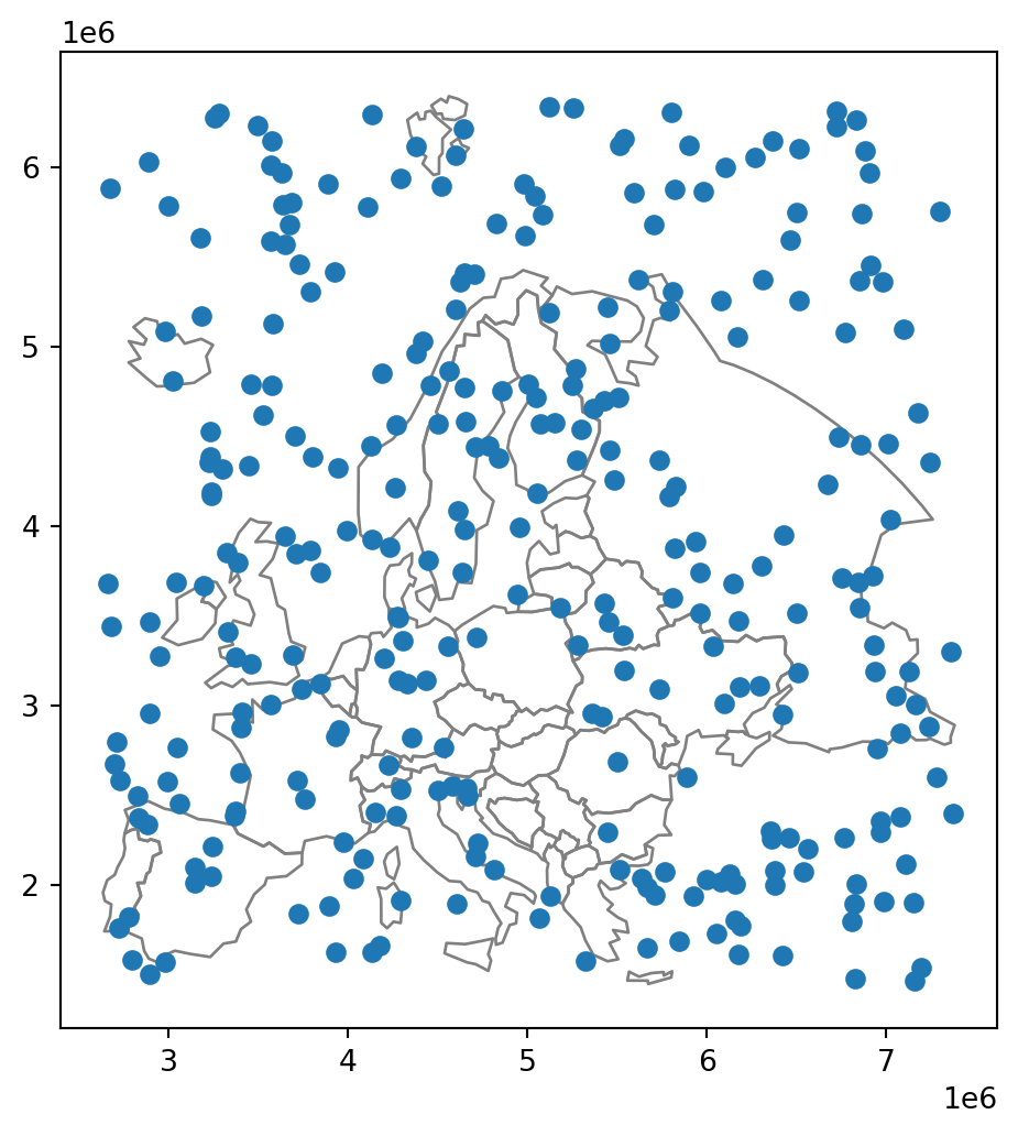
europe
New geometries
geopandas contains numerous properties and methods to calculate new geometries, based on the input geometries contained in a GeoSeries or a GeoDataFrame, implementing various useful spatial analysis algorithms. For example, the .centroid property returns the centroids of the input geometries:
europe.centroid0 POINT (5164278.053 2059887.807)
1 POINT (4626259.985 2731530.423)
2 POINT (5498997.072 3523529.622)
...
36 POINT (5847697.706 3120841.915)
37 POINT (3485900.377 3485242.948)
38 POINT (6209366.017 4042511.414)
Length: 39, dtype: geometryNote that the result of .centroid (and similar methods) is returned in the form of a GeoSeries, even when the input is a GeoDataFrame!
Figure 4.12 shows both the input europe and the calculated centroids europe.centroid:
base = europe.plot(color='none', edgecolor='lightgrey')
europe.centroid.plot(ax=base);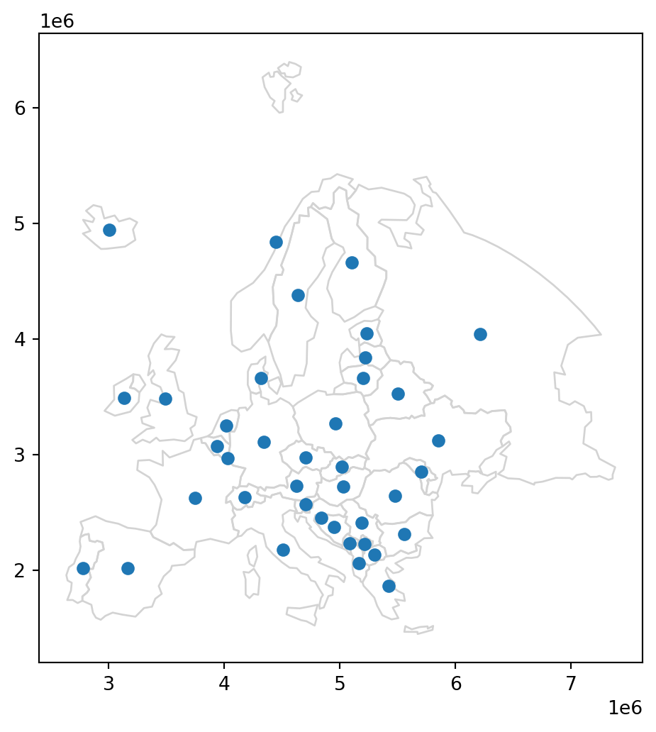
Note
shapely and geopandas assume planar CRS, even when a geographical CRS is specified (in geopandas). Therefore, when doing spatial calculations (such as .centroid, .area, etc.), make sure that the input layer(s) are in a projected CRS!
The .envelope property returns the bounding box polygons of the given geometries, as demonstrated in Figure 4.13:
base = europe.plot(color='none', edgecolor='lightgrey')
europe.envelope.plot(ax=base, color='none', edgecolor='C0');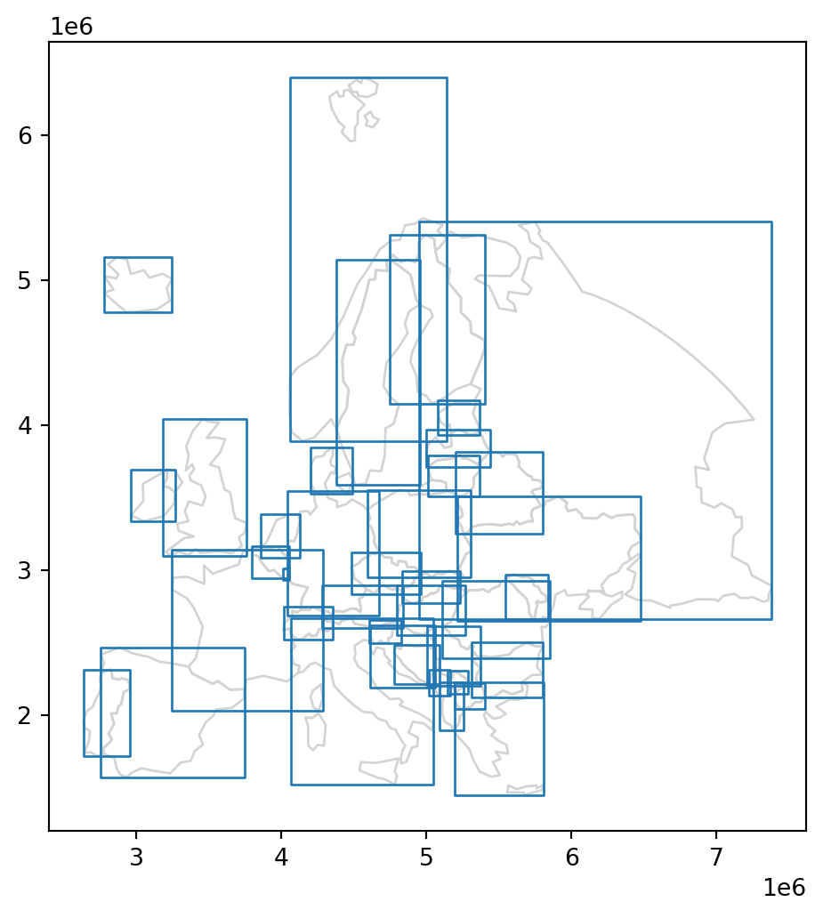
The .buffer method returns buffered geometries, to the specified distance (in CRS units!). For example, Figure 4.14 shows 100 \(km\) buffers around European countries:
base = europe.plot(color='none', edgecolor='lightgrey')
europe.buffer(100_000).plot(ax=base, color='none', edgecolor='C0');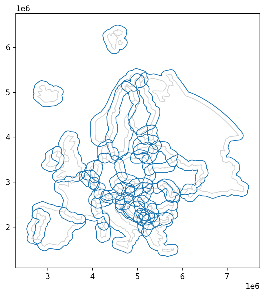
Dissolving
The .union_all method returns the union of all input geometries. In the case of polygons, the inputs are therefore combined and also “dissolved”. For example:
europe1 = europe.union_all()Note that .union_all returns a single shapely geometry (Figure 4.15). Consequently, the attributes of the input geometries (if any) are lost:
europe1
.union_all
If we need to go back to geopandas representation of the resulting geometry for further anyalysis, writing to file, etc., then we can convert it to a GeoSeries of length 1, as follows. Note that we also need to “restore” the CRS, which was also lost in the transition to shapely:
europe1 = gpd.GeoSeries(europe1, crs=europe.crs)
europe1
0 MULTIPOLYGON (((4183464.723 192...
dtype: geometryFigure 4.16 shows the dissolved countries, now in a GeoSeries:
base = europe.plot(color='none', edgecolor='lightgrey')
europe1.plot(ax=base, color='none', edgecolor='C0');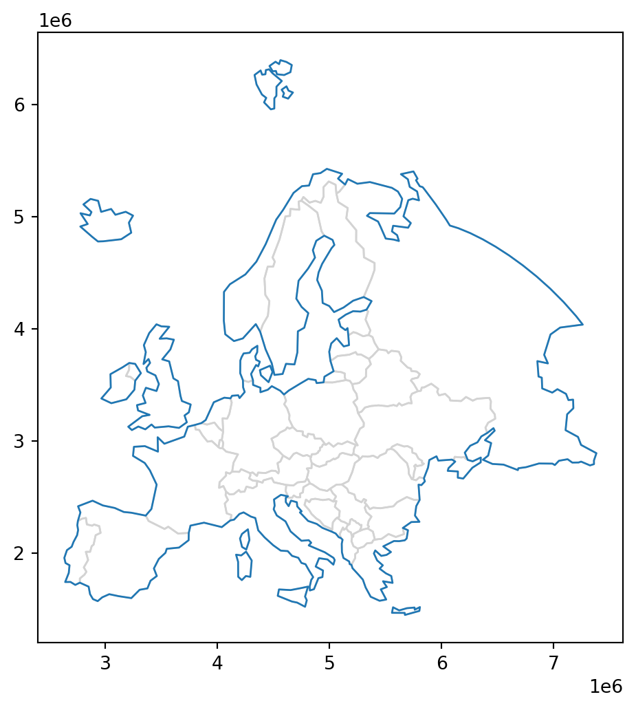
Spatial relations (geopandas)
geopandas contains numerous functions to evaluate pairwise relations between geometries. The methods are analogous to the shapely methods (Spatial relations (shapely)). However, the geopandas methods can be applied to all geometries in a GeoSeries or a GeoDataFrame, contrasted with an individual “fixed” shapely geometry. The result is a boolean Series specifying whether each of the input geometries intersects with the individual geometry.
For example, suppose we have the europe layer of European countries, and an individual shapely geometry of Spain (Figure 4.17):
spain = europe[europe['name'] == 'Spain'].geometry.iloc[0]
spain
shapely polygon geometry of Spain
Here is how we can evaluate whether each country in europe intersects with spain:
sel = europe.intersects(spain)
sel
0 False
1 False
2 False
...
36 False
37 False
38 False
Length: 39, dtype: boolThe boolean series sel can be used for subsetting, if necessary:
europe[sel]| name | geometry | |
|---|---|---|
| 11 | France | MULTIPOLYGON (((4271123.887 221... |
| 28 | Portugal | POLYGON ((2754169.742 2285654.7... |
| 33 | Spain | POLYGON ((2771755.985 1735745.1... |
Figure 4.18 demonstrates the subsetting operation:
base = europe.plot(edgecolor='grey', color='none')
europe[sel].plot(ax=base, edgecolor='none', color='pink')
europe[europe['name'] == 'Spain'].plot(ax=base, edgecolor='red', color='none');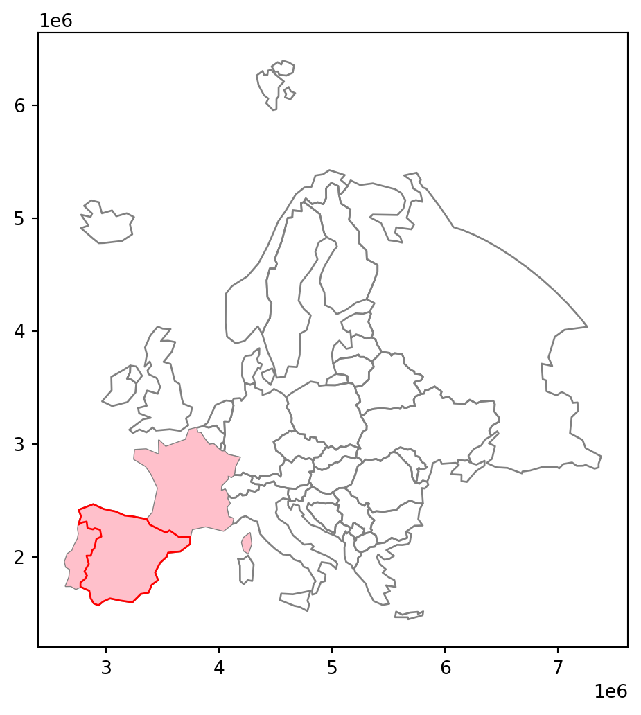
geopandas: a polygon layer of countries (in grey), a geometry used for subsetting (Spain, in red), and the resulting subset of countries intersecting with that geometry (France, Portugal, and Spain, in pink)
Practice
- Write an expression that returns the count of
pointswhich intersect with theeuropegeometries.
Creating regular grids
When evaluating and mapping accessibility through spatial network (Accessibility), we are often required to create a regular grid covering the studied area. That way, we can calculate and display a continuous surface of estimates for the given metric, such as travel time to a fixed location (e.g., Figure 19.23). Since creating a regular grid is going to be a repetitive task, we are going to define a function named create_grid to automate this step.
The create_grid is defined (Function definition) in the net2 module (Custom modules), as follows. We are not going to go over all of the details on how the function works. You may notice that some of the code uses principles explained in the last two chapters:
def create_grid(bounds, res, crs=None):
    xmin, ymin, xmax, ymax = bounds
    cols = list(np.arange(int(np.floor(xmin)), int(np.ceil(xmax+res)), res))
    rows = list(np.arange(int(np.floor(ymin)), int(np.ceil(ymax+res)), res))
    rows.reverse()
    polygons = []
    for x in cols:
        for y in rows:
            polygons.append(
                shapely.Polygon([(x,y), (x+res, y), (x+res, y-res), (x, y-res)])
            )
    grid = gpd.GeoDataFrame({'geometry': polygons}, crs=crs)
    sel = grid.intersects(shapely.box(*bounds))
    grid = grid[sel]
    return grid
Note that the function is named create_grid. The above definition is placed in the net.py script, which we can import using the expression import net2, and subsequently call using net2.create_grid.
Let’s demonstrate how the function can be used. In the example, we create a regular grid covering the extent of roads minus 1500 \(m\) (i.e., a negative buffer), at 1000 \(m\) resolution. Here are the setting we need to specify:
bounds = roads.union_all().envelope.buffer(-1500).bounds
res = 1000
crs = roads.crs
These three objects can be passed to net2.create_grid, as follows. The resulting object—which we assign to grid—is a GeoDataFrame of grid cells:
grid = net2.create_grid(bounds, res, crs)
grid| geometry | |
|---|---|
| 0 | POLYGON ((667633 3464160, 66863... |
| 1 | POLYGON ((667633 3463160, 66863... |
| 2 | POLYGON ((667633 3462160, 66863... |
| ... | ... |
| 62 | POLYGON ((672633 3457160, 67363... |
| 63 | POLYGON ((672633 3456160, 67363... |
| 64 | POLYGON ((672633 3455160, 67363... |
60 rows × 1 columns
Figure 4.19 shows the result:
base = roads.plot(zorder=0, color='lightgrey')
grid.plot(ax=base, color='none', zorder=1);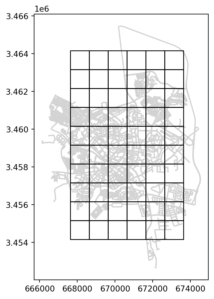
net2.create_grid
Pairwise matrices
Pairwise matrices quantifying the relations between spatial entities can be naturally represented using a spatial network. Think of a distance matrix between locations, or a migration flow matrix between countries. As an example, we are going to create a matrix representing shared borders between European countries.
Figure 5.10 shows the europe polygonal layer which we start from:
europe.plot(edgecolor='black', color='lightgrey');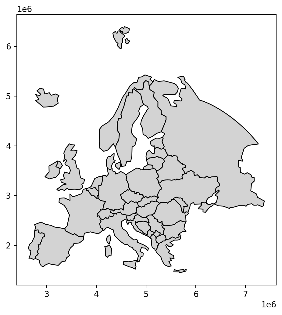
First, we transfer the 'name' column to the rows index (Setting the index). That way, the names are going to appear in the resulting matrix row and column indices:
europe = europe.set_index('name')
europe| geometry | |
|---|---|
| name | |
| Albania | POLYGON ((5250878.03 2039389.75... |
| Austria | POLYGON ((4839987.968 2803428.6... |
| Belarus | POLYGON ((5436932.506 3816251.1... |
| ... | ... |
| Ukraine | POLYGON ((5788113.051 3443307.2... |
| United Kingdom | MULTIPOLYGON (((3455660.833 344... |
| Russia | MULTIPOLYGON (((7174520.945 329... |
39 rows × 1 columns
Then, we use .apply to repeatedly run .intersects (Spatial relations (geopandas)) and obtain a complete matrix m:
m = europe.apply(lambda x: europe.intersects(x.geometry), axis=1)
m| name | Albania | Austria | Belarus | Belgium | Bosnia and Herz. | ... | Sweden | Switzerland | Ukraine | United Kingdom | Russia |
|---|---|---|---|---|---|---|---|---|---|---|---|
| name | |||||||||||
| Albania | True | False | False | False | False | ... | False | False | False | False | False |
| Austria | False | True | False | False | False | ... | False | True | False | False | False |
| Belarus | False | False | True | False | False | ... | False | False | True | False | True |
| ... | ... | ... | ... | ... | ... | ... | ... | ... | ... | ... | ... |
| Ukraine | False | False | True | False | False | ... | False | False | True | False | True |
| United Kingdom | False | False | False | False | False | ... | False | False | False | True | False |
| Russia | False | False | True | False | False | ... | False | False | True | False | True |
39 rows × 39 columns
Note
Usage of .apply is beyond the scope of this book. For more information, check the pandas documentation and the and the distance calculation example from Introduction to Spatial Data Programming with Python.
We can remove the axis names, to make the matrix more simple:
m = m.rename_axis(None, axis=0)
m = m.rename_axis(None, axis=1)
m| Albania | Austria | Belarus | Belgium | Bosnia and Herz. | ... | Sweden | Switzerland | Ukraine | United Kingdom | Russia | |
|---|---|---|---|---|---|---|---|---|---|---|---|
| Albania | True | False | False | False | False | ... | False | False | False | False | False |
| Austria | False | True | False | False | False | ... | False | True | False | False | False |
| Belarus | False | False | True | False | False | ... | False | False | True | False | True |
| ... | ... | ... | ... | ... | ... | ... | ... | ... | ... | ... | ... |
| Ukraine | False | False | True | False | False | ... | False | False | True | False | True |
| United Kingdom | False | False | False | False | False | ... | False | False | False | True | False |
| Russia | False | False | True | False | False | ... | False | False | True | False | True |
39 rows × 39 columns
The matrix can be exported to a CSV file named 'europe_borders.csv', which we are going to use later on in the book:
m.to_csv('output/europe_borders.csv')When importing the matrix back into a DataFrame, we specify index_col=0 to make sure that the first column is interpreted as the row indices, rather than as an “ordinary” column:
pd.read_csv('output/europe_borders.csv', index_col=0)| Albania | Austria | Belarus | Belgium | Bosnia and Herz. | ... | Sweden | Switzerland | Ukraine | United Kingdom | Russia | |
|---|---|---|---|---|---|---|---|---|---|---|---|
| Albania | True | False | False | False | False | ... | False | False | False | False | False |
| Austria | False | True | False | False | False | ... | False | True | False | False | False |
| Belarus | False | False | True | False | False | ... | False | False | True | False | True |
| ... | ... | ... | ... | ... | ... | ... | ... | ... | ... | ... | ... |
| Ukraine | False | False | True | False | False | ... | False | False | True | False | True |
| United Kingdom | False | False | False | False | False | ... | False | False | False | True | False |
| Russia | False | False | True | False | False | ... | False | False | True | False | True |
39 rows × 39 columns
Rasters with rasterio
Reading raster from file
Note
This section introduces the rasterio package for working with rasters. We are only going to work with rasters in one of the later chapters Raster least cost paths. You can skip this section for now, and return to it when reaching the latter chapter.
The rasterio package works with the concept of a file connection. A raster file connection has two components:
- The metadata (such as the dimensions, resolution, CRS, etc.)
- A reference to the raster values
When necessary, the values can be read into memory, either all at once, or from a particular band and/or “window”, or at a particular resolution. The rationale is that the metadata are small (and often useful to examine on their own), while values are often very big. Therefore, it can be more practical to have control over which values to read, and when.
To create a file connection object to a raster file, we use the rasterio.open function. For example, here we create a file connection object named src, which refers to the dem.tif raster. This is a Digital Elevation Model (DEM) of the Grand Canyon:
src = rasterio.open('data/dem.tif')
src
<open DatasetReader name='data/dem.tif' mode='r'>The raster metadata can be accessed through the .src property of the file connection. For example, from the following metadata object:
src.meta{'driver': 'GTiff',
'dtype': 'float32',
'nodata': None,
'width': 250,
'height': 250,
'count': 1,
'crs': CRS.from_wkt('PROJCS["WGS 84 / UTM zone 12N",GEOGCS["WGS 84",DATUM["WGS_1984",SPHEROID["WGS 84",6378137,298.257223563,AUTHORITY["EPSG","7030"]],AUTHORITY["EPSG","6326"]],PRIMEM["Greenwich",0,AUTHORITY["EPSG","8901"]],UNIT["degree",0.0174532925199433,AUTHORITY["EPSG","9122"]],AUTHORITY["EPSG","4326"]],PROJECTION["Transverse_Mercator"],PARAMETER["latitude_of_origin",0],PARAMETER["central_meridian",-111],PARAMETER["scale_factor",0.9996],PARAMETER["false_easting",500000],PARAMETER["false_northing",0],UNIT["metre",1,AUTHORITY["EPSG","9001"]],AXIS["Easting",EAST],AXIS["Northing",NORTH],AUTHORITY["EPSG","32612"]]'),
'transform': Affine(30.0, 0.0, 340150.5054945286,
0.0, -30.0, 4025687.7291128924)}we can learn that:
- Raster data type is 32-bit float (
float32) - Raster size is \(250 \times 250\) pixels
- Raster has 1 band
- Raster CRS is UTM Zone 12N (EPSG:32612)
- Raster resolution is 30 \(m\)
The raster values can be read using the .read method. The default is to read all values (as mentioned above, there are many other options to read partial data):
r = src.read()
r
array([[[1703.5546 , 1699.9779 , 1691.0651 , ..., 885.72205,
838.30835, 772.8654 ],
[1704.1259 , 1695.7571 , 1686.433 , ..., 821.11163,
807.0282 , 763.33026],
[1699.1866 , 1687.0507 , 1672.4417 , ..., 750.7814 ,
758.62134, 736.97504],
...,
[1226.0349 , 1230.9957 , 1231.9414 , ..., 1295.1006 ,
1293.3195 , 1293.5986 ],
[1221.9559 , 1227.7778 , 1229.0176 , ..., 1294.4015 ,
1294.5459 , 1295.1248 ],
[1218.4246 , 1225.5681 , 1225.654 , ..., 1292.4885 ,
1294.6091 , 1296.3708 ]]], shape=(1, 250, 250), dtype=float32)r = src.read(1)
rarray([[1703.5546 , 1699.9779 , 1691.0651 , ..., 885.72205, 838.30835,
772.8654 ],
[1704.1259 , 1695.7571 , 1686.433 , ..., 821.11163, 807.0282 ,
763.33026],
[1699.1866 , 1687.0507 , 1672.4417 , ..., 750.7814 , 758.62134,
736.97504],
...,
[1226.0349 , 1230.9957 , 1231.9414 , ..., 1295.1006 , 1293.3195 ,
1293.5986 ],
[1221.9559 , 1227.7778 , 1229.0176 , ..., 1294.4015 , 1294.5459 ,
1295.1248 ],
[1218.4246 , 1225.5681 , 1225.654 , ..., 1292.4885 , 1294.6091 ,
1296.3708 ]], shape=(250, 250), dtype=float32)The resulting object r is an ndarray object (package numpy):
type(r)numpy.ndarrayThe array stores the values using the same data type and the same precision as in the original file:
r.dtypedtype('float32')This means that the minimal amount of RAM is being used, which is an advantage of Python over other programming languages such as R.
Graphics: rasterio
The rasterio.plot.show function—from the rasterio.plot “sub-package”—can be used to plot a raster. This function can accept, and read from, a file connection (Figure 4.21):
rasterio.plot.show(src);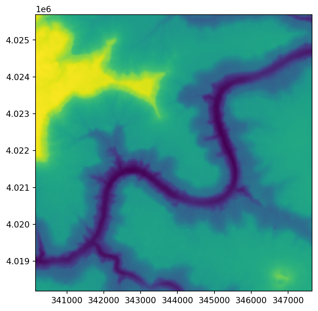
Plotting a point on top of a raster, using numeric coordinates, can be done as follows (Figure 4.22):
fig, ax = plt.subplots()
rasterio.plot.show(src, ax=ax)
plt.plot(345000, 4025000, 'ro');
plt.plot
A GeoSeries (or GeoDataFrame), in this case also a point, can be added to a raster plot as follows (Figure 4.23):
fig, ax = plt.subplots()
rasterio.plot.show(src, ax=ax)
gpd.GeoSeries([shapely.Point(345000, 4025000)]).plot(color='red', ax=ax);
GeoSeries
Pixel values
Once they are imported into the Python environment, we can work with raster values just like with any other ndarray object. For example, here is how we can access the value of a specific raster pixel, in this case—the top-left corner:
r[0,0]np.float32(1703.5546)Here is how we can calculate the minimum and the maximum pixel values:
np.min(r)np.float32(549.84973)np.max(r)np.float32(1754.025)Transformation matrix
The main difference between a plain array and a raster is that the raster is georeferenced. In rasterio, the georeferencing information can be accessed through the transformation matrix, in the .transform property:
src.transformAffine(30.0, 0.0, 340150.5054945286,
0.0, -30.0, 4025687.7291128924)The matrix stores the raster origin (top-left coordinate) xmin,ymax, and resolution delta_x,delta_y, as follows:
Affine(delta_x, 0.0,     xmin,
       0.0,     delta_y, ymax)
Therefore, the origin of the 'dem.tif' raster is:
transform = src.transform
transform[2], transform[5]
(340150.5054945286, 4025687.7291128924)and the resolution is:
transform[0], transform[4](30.0, -30.0)Pixel coordinates
The information in the transformation matrix is sufficient to calculate the coordinates of all raster pixels. Starting from the origin, we add the resolution as many times as necessary–according to the number of steps to go through the rows and columns—adding half a pixel size in the end to get the pixel center coordinates. rasterio provides an automatic method to do that, i.e., to get pixel centroid coordinates given the row and column indices.
First, we pass the transformation matrix object to the rasterio.transform.AffineTransformer function. The result is a transformer function, specific to the given raster, hereby named transformer:
transformer = rasterio.transform.AffineTransformer(src.transform)
transformer<AffineTransformer>Then, the transformer function can be used to calculate the coordinates of any given pixel. For example, here are the coordinates of the centroid of the top-left pixel:
row, col = 0, 0
transformer.xy(row, col)
(np.float64(340165.5054945286), np.float64(4025672.7291128924))For comparison, here is how we could “manually” calculate the same coordinates:
src.transform[2] + src.transform[0] * row + src.transform[0]/2, \
src.transform[5] + src.transform[4] * col + src.transform[4]/2
(340165.5054945286, 4025672.7291128924)Exercises
Exercise 03-01
- Select one European country
- Plot the selected country borders, together with three buffer sizes—100 \(km\), 200 \(km\), and 300 \(km\) (Figure 19.1)
Exercise 03-02
- Select one European country
- Calculate the distances, in \(km\), from the selected country to all other European countries (excluding self)
- Print a table of with the names and distances of the 10 nearest countries, sorted by ascending distance (Table 19.2)
Exercise 03-03
- Find the location of the lowest point of the raster and plot the raster with that location marked (Figure 19.2)
- Tip: use
np.argminandnp.unravel_indexto find the row and column of the minimal value in a two-dimensional raster