Last updated: 2026-03-04 01:42:59Multiple locations
Introduction
In this chapter we demonstrate operations related to accessibility to a set of several locations, rather than just one:
First, we repeat the previous material of preparing network data (Pre-processing) and a regular grid (Negev grid), and then calculating accessibility to one location (Negev accessibility), but this time using a road network of a larger area (Negev network)
Once the network data are ready we introduce two new types of routing calculations involving more than one location:
- We calculate a travel time matrix coverig all pairs of several locations (Travel time matrix)
- We calculate maps of accessibility and optimal allocation to the nearest location (Optimal allocation)
Packages
import numpy as np
import pandas as pd
import matplotlib.pyplot as plt
import shapely
import geopandas as gpd
import networkx as nx
import osmnx as ox
import pyproj
import net2
Negev network
For the examples in this chapter, we prepare a road network of the Beer-Sheba sub-district in Israel:
G = ox.graph_from_place('Beersheba Subdistrict, Israel', network_type='drive', truncate_by_edge=True)
G
<networkx.classes.multidigraph.MultiDiGraph at 0x7dd7cf5aa180>Pre-processing
Let’s make the network object routable, following the same steps we went through in OpenStreetMap and osmnx.
First, we add the travel times (Imputing travel times):
G = ox.add_edge_speeds(G)
G = ox.add_edge_travel_times(G)
Figure 12.1 is a map of the edge speeds:
edges = net2.edges_to_gdf(G)
base = edges.plot(column='speed_kph', legend=True, cmap='Spectral_r', linewidth=0.8)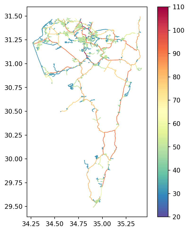
Next we simplify the network from a MultiDiGraph to a DiGraph:
G = ox.convert.to_digraph(G, weight='travel_time')
G
<networkx.classes.digraph.DiGraph at 0x7dd7d2ff93a0>We apply the net2.prepare function to validate and standardize the attributes (Standardizing the network):
G = net2.prepare(G)
G
<networkx.classes.digraph.DiGraph at 0x7dd7d09f6000>Next, we fill node geometries and missing edge geometries (Filling edge geometries):
for i in G.nodes:
    G.nodes[i]['geometry'] = shapely.Point(G.nodes[i]['x'], G.nodes[i]['y'])
for u,v in G.edges:
    e = G.edges[u, v]
    if 'geometry' not in e:
        geom = shapely.LineString([G.nodes[u]['geometry'], G.nodes[v]['geometry']])
        G[u][v]['geometry'] = geom
We delete the unnecessary attributes:
keep = ['geometry']
for i in G.nodes:
    for attr in list(G.nodes[i].keys()):
        if attr not in keep:
            del G.nodes[i][attr]
keep = ['geometry', 'length', 'speed_kph', 'time']
for u,v in G.edges:
for attr in list(G.edges[u,v].keys()):
if attr not in keep:
del G.edges[u,v][attr]Finally, we transform the coordinates to a projected CRS (Projecting geometries):
transformer = pyproj.Transformer.from_crs(4326, 32636, always_xy=True)
for i in G.nodes:
    G.nodes[i]['geometry'] = shapely.transform(
        G.nodes[i]['geometry'],
        transformer.transform,
        interleaved=False
    )
for u,v in G.edges:
    G.edges[u, v]['geometry'] = shapely.transform(
        G.edges[u, v]['geometry'],
        transformer.transform,
        interleaved=False
    )
Writing the Negev network
To use the Negev network elsewhere, let’s export it to an '.xml' file:
H = G.copy()
for i in H.nodes:
    H.nodes[i]['geometry'] = str(H.nodes[i]['geometry'])
for u,v in H.edges:
    H.edges[u, v]['geometry'] = str(H.edges[u, v]['geometry'])
nx.write_graphml(H, 'output/negev.xml')
Negev grid
Let’s also create a regular grid for accessibility calculations. Here, we are making a \(15 \times 15\) \(km^2\) grid, covering the road network extent buffered by \(5\) \(km\):
edges = net2.edges_to_gdf(G)
bounds = edges.buffer(5000).total_bounds
grid = net2.create_grid(bounds, 15000, 32636)
grid| geometry | |
|---|---|
| 0 | POLYGON ((615570 3498877, 63057... |
| 1 | POLYGON ((615570 3483877, 63057... |
| 2 | POLYGON ((615570 3468877, 63057... |
| ... | ... |
| 132 | POLYGON ((720570 3303877, 73557... |
| 133 | POLYGON ((720570 3288877, 73557... |
| 134 | POLYGON ((720570 3273877, 73557... |
128 rows × 1 columns
Figure 12.2 shows the grid on top of the road network:
base = grid.plot(color='none', edgecolor='grey')
edges.plot(ax=base, color='red', linewidth=0.5);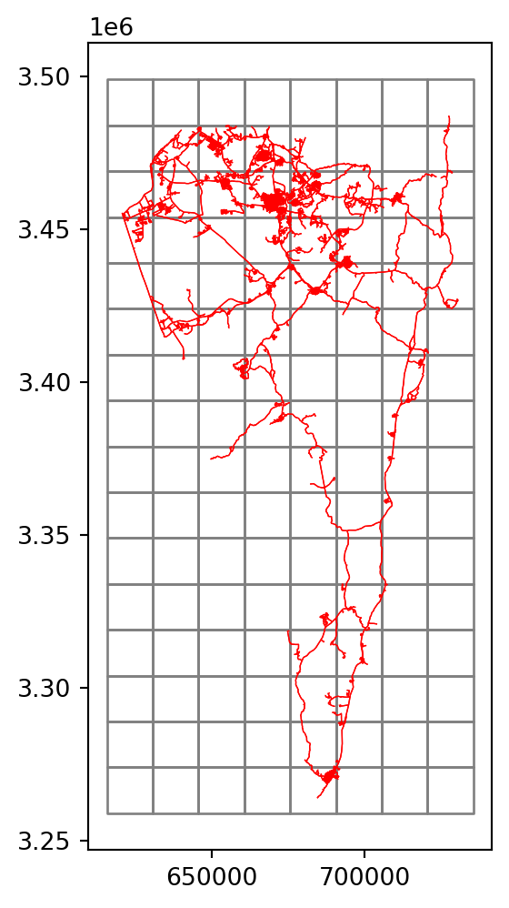
As you can see in Figure 12.2, much of the grid is far from any road (and actually even beyond the country borders). Assuming we are not interested in accessibility to those remote locations, let’s filter the grid according to intersection with the roads plus a \(1\) \(km\) buffer:
grid = grid[grid.intersects(edges.buffer(1000).union_all())]
grid| geometry | |
|---|---|
| 1 | POLYGON ((615570 3483877, 63057... |
| 2 | POLYGON ((615570 3468877, 63057... |
| 3 | POLYGON ((615570 3453877, 63057... |
| ... | ... |
| 123 | POLYGON ((720570 3438877, 73557... |
| 124 | POLYGON ((720570 3423877, 73557... |
| 125 | POLYGON ((720570 3408877, 73557... |
76 rows × 1 columns
Figure 12.3 shows the filtered grid:
base = grid.plot(color='none', edgecolor='grey')
edges.plot(ax=base, color='red', linewidth=0.5);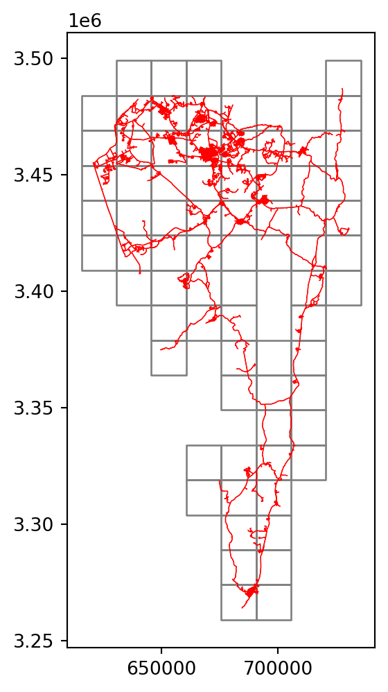
Finally, we calculate the grid cell centroids, which are going to be used for routing:
ctr = grid.centroid
ctr
1 POINT (623070 3476377)
2 POINT (623070 3461377)
3 POINT (623070 3446377)
...
123 POINT (728070 3431377)
124 POINT (728070 3416377)
125 POINT (728070 3401377)
Length: 76, dtype: geometryFigure 12.4 shows the centroids:
base = grid.plot(color='none', edgecolor='lightgrey', zorder=0)
edges.plot(ax=base, color='red', linewidth=0.5, zorder=1)
ctr.plot(color='black', markersize=5, ax=base, zorder=2);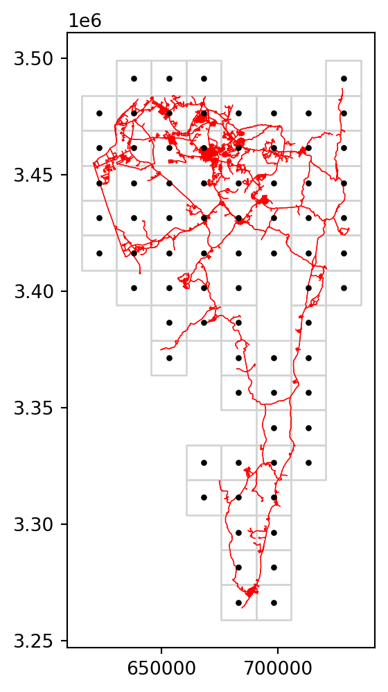
Negev accessibility
Now let’s calculate an accessibility map to a specific location in Beer-Sheva. First we define the coordinates pnt:
pnt = shapely.Point(34.799796, 31.281758)  # Ramot Sportiv
pnt = shapely.transform(pnt, transformer.transform, interleaved=False)
pnt
Then, we go over the centroids and each time calculate the travel time:
result = []
for i in ctr.to_list():
    result.append(net2.route2(G, pnt, i, 'time')['weight'])
grid['time'] = result
grid| geometry | time | |
|---|---|---|
| 1 | POLYGON ((615570 3483877, 63057... | 5376.124498 |
| 2 | POLYGON ((615570 3468877, 63057... | 3427.653311 |
| 3 | POLYGON ((615570 3453877, 63057... | 3857.947577 |
| ... | ... | ... |
| 123 | POLYGON ((720570 3438877, 73557... | 3344.819324 |
| 124 | POLYGON ((720570 3423877, 73557... | 3876.807474 |
| 125 | POLYGON ((720570 3408877, 73557... | 5044.281401 |
76 rows × 2 columns
Figure 12.5 shows the map of calculated travel times:
base = grid.plot(column='time', cmap='Spectral', legend=True)
net2.edges_to_gdf(G).plot(ax=base, linewidth=0.1, color='black')
plt.plot(pnt.x, pnt.y, 'ro');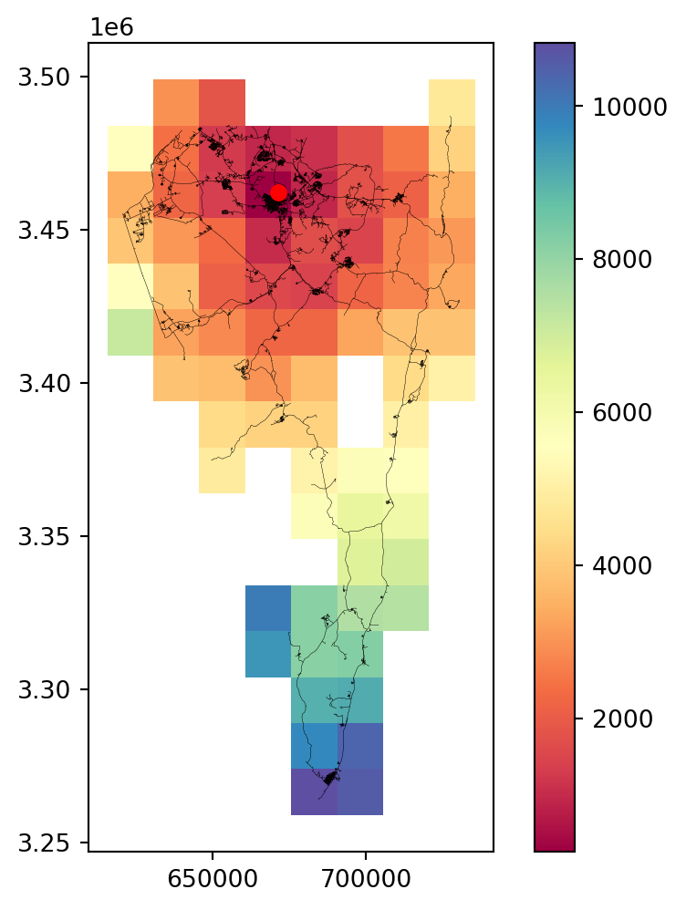
Travel time matrix
List of locations
In the next example, we evaluate all pairwise travel times between locations, to create a “travel time matrix”.
First, we define our locations of interest:
locations = ['Eilat', 'Beer-Sheva', 'Ein Gedi', 'Sde Boker']
locations
['Eilat', 'Beer-Sheva', 'Ein Gedi', 'Sde Boker']Then, we use gecoding to get the locations’ coordinates:
pnt = [ox.geocoder.geocode(i) for i in locations]
pnt = [(i[1], i[0]) for i in pnt]
pnt = [shapely.Point(i) for i in pnt]
pnt
[<POINT (34.945 29.554)>,
<POINT (34.793 31.246)>,
<POINT (35.385 31.452)>,
<POINT (34.793 30.874)>]We transform the coordinates to UTM, so that they are in agreement with the network:
pnt = [shapely.transform(i, transformer.transform, interleaved=False) for i in pnt]
pnt
[<POINT (688469.178 3270948.471)>,
<POINT (670697.192 3458222.402)>,
<POINT (726617.896 3482202.305)>,
<POINT (671370.351 3416985.166)>]Let’s also collect the coordinates to a GeoSeries:
geom = gpd.GeoSeries(pnt, crs=32636)
geom
0 POINT (688469.178 3270948.471)
1 POINT (670697.192 3458222.402)
2 POINT (726617.896 3482202.305)
3 POINT (671370.351 3416985.166)
dtype: geometryNow we can plot the locations GeoSeries named geom, with text labels (Figure 12.6):
base = edges.plot(color='grey', linewidth=0.2, zorder=0)
geom.plot(color='blue', markersize=50, ax=base)
for i in zip(locations, pnt):
    base.annotate(i[0], (i[1].x, i[1].y), ha='left', weight='bold');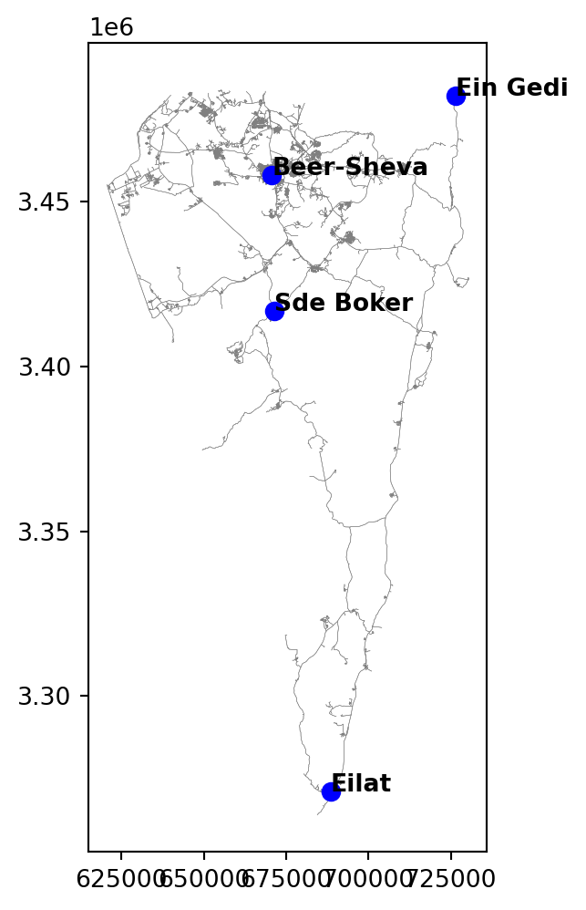
Individual route
As an example, here is how we calculate the fastest route from Beer-Sheva to Eilat:
x = net2.route2(G, pnt[1], pnt[0], 'time') # Beer-Sheva to EilatWe can transform the route to a GeoDataFrame:
route = net2.route_to_gdf(x['network'], x['route'])and display it on a map (Figure 12.7):
base = edges.plot(color='grey', linewidth=0.2, zorder=0)
geom.plot(color='blue', markersize=50, ax=base, zorder=1)
route.plot(ax=base, color='red', zorder=2)
for i in zip(locations, pnt):
    base.annotate(i[0], (i[1].x, i[1].y), ha='left', weight='bold');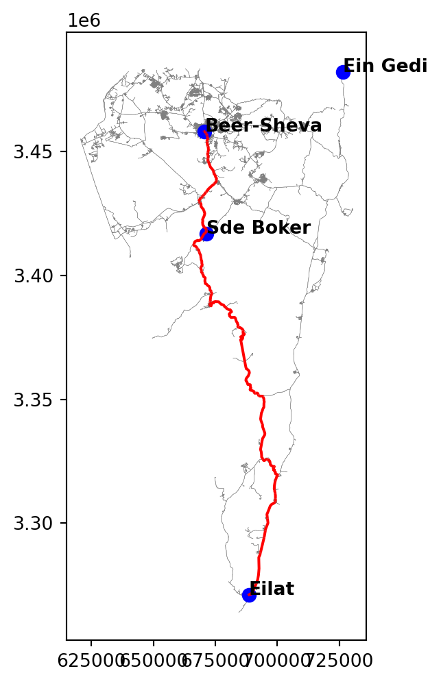
All routes
Now, let’s systematically calculate all pairwise routes between the locations, and collect them into a travel time matrix.
First, we create a template matrix, initially filled with zeros:
result = np.zeros([len(locations), len(locations)])
result
array([[0., 0., 0., 0.],
[0., 0., 0., 0.],
[0., 0., 0., 0.],
[0., 0., 0., 0.]])Now, we execute two nested for loops, each going over the indices of the locations. Inside the internal loop, for each pair of indices i and j, we calculate the fastest route, and extract the summed weight (i.e., total travel time) into the corresponding cell of the matrix result[i,j]:
for i in range(len(locations)):
    for j in range(len(locations)):
        result[i,j] = net2.route2(G, pnt[i], pnt[j], 'time')['weight']
In the end, we have a travel time matrix with values in \(sec\):
resultarray([[ 0. , 10273.1930297 , 10293.98976859, 8345.90716181],
[10237.29794896, 0. , 4548.05015518, 2016.63624164],
[10321.9738277 , 4533.37628218, 0. , 5571.27254429],
[ 8325.23514752, 2030.74607572, 5573.60512156, 0. ]])Let’s transform it from seconds to hours:
result = result * (1/60) * (1/60)
result
array([[0. , 2.85366473, 2.8594416 , 2.31830754],
[2.84369387, 0. , 1.26334727, 0.56017673],
[2.86721495, 1.25927119, 0. , 1.54757571],
[2.31256532, 0.56409613, 1.54822364, 0. ]])To examine the results more easily, we can transform the matrix (ndarray) to a table (DataFrame) while adding row and column labels with location names:
dat = pd.DataFrame(result, index=locations, columns=locations)
dat| Eilat | Beer-Sheva | Ein Gedi | Sde Boker | |
|---|---|---|---|---|
| Eilat | 0.000000 | 2.853665 | 2.859442 | 2.318308 |
| Beer-Sheva | 2.843694 | 0.000000 | 1.263347 | 0.560177 |
| Ein Gedi | 2.867215 | 1.259271 | 0.000000 | 1.547576 |
| Sde Boker | 2.312565 | 0.564096 | 1.548224 | 0.000000 |
A travel time matrix can be translated “back” to a spatial network (e.g., Figure 19.27). The entire workflow can then be thought of as “simplification” of the network, keeping just the relevant nodes, and discarding or merging the edges accordingly. The simplified network can then be subject to further processing, for example algorithms such as the Traveling Salesman Problem (see Exercise 11-03).
Optimal allocation
In the following example, we are going to calculate and map optimal allocation to a given set facilities. In this example, we calculate the allocation of each grid cell in the Negev to one of the two hospitals in the area—Soroka and Yoseftal. Each grid cell is going to be allocated to one of the hospitals, according to optimal (shortest) travel time.
First, let’s define the facility locations:
locations = ['Soroka Hospital', 'Yoseftal Hospital']
locations
['Soroka Hospital', 'Yoseftal Hospital']and calculate their coordinates through geocoding (Geocoding (osmnx)) and reprojection (Reprojection (shapely)):
pnt = [ox.geocoder.geocode(i) for i in locations]
pnt = [(i[1], i[0]) for i in pnt]
pnt = [shapely.Point(i) for i in pnt]
pnt = [shapely.transform(i, transformer.transform, interleaved=False) for i in pnt]
pnt
[<POINT (671476.109 3459617.482)>, <POINT (688011.999 3270955.999)>]Figure 12.8 shows the locations of the Soroka and Yoseftal hospitals. To display the points, we first transform them from a list of coordinate pairs to a GeoSeries:
geom = gpd.GeoSeries([shapely.Point(i) for i in pnt])
geom
0 POINT (671476.109 3459617.482)
1 POINT (688011.999 3270955.999)
dtype: geometryand then plot (Figure 12.8):
base = grid.plot(color='none', edgecolor='grey')
ctr.plot(color='grey', markersize=1, ax=base)
geom.plot(color='red', markersize=50, ax=base);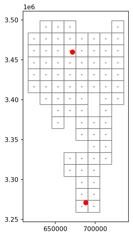
Now we calculate the accessibility to all—i.e., two, in this case—facilities. Note the internal loop with index j, where we go over the location indices. Inside that loop, we calculate a list times1 with the corresponding travel times to all facilities. Then, we extract the minimum times into the list named times, and the indices of the minimum times into another list named ids. These two lists are then transferred into the columns named h_time and h_id, respectively:
times = []
ids = []
for i in ctr.to_list():
    times1 = []
    for j in range(len(locations)):
        times1.append(net2.route2(G, pnt[j], i, 'time')['weight'])
    times.append(min(times1))
    ids.append(times1.index(min(times1)))
grid['h_time'] = times
grid['h_id'] = ids
grid| geometry | time | h_time | h_id | |
|---|---|---|---|---|
| 1 | POLYGON ((615570 3483877, 63057... | 5376.124498 | 5431.891438 | 0 |
| 2 | POLYGON ((615570 3468877, 63057... | 3427.653311 | 3483.420251 | 0 |
| 3 | POLYGON ((615570 3453877, 63057... | 3857.947577 | 3913.714517 | 0 |
| ... | ... | ... | ... | ... |
| 123 | POLYGON ((720570 3438877, 73557... | 3344.819324 | 3313.910233 | 0 |
| 124 | POLYGON ((720570 3423877, 73557... | 3876.807474 | 3845.898383 | 0 |
| 125 | POLYGON ((720570 3408877, 73557... | 5044.281401 | 5013.372311 | 0 |
76 rows × 4 columns
Figure 12.9 shows the results in the h_time column—the travel time to the nearest hospital. Note that the resulting surface has just two possible values as there are two facilities that can be nearest: 0 for Soroka and 1 for Yoseftal:
base = grid.plot(column='h_time', cmap='Spectral', legend=True, zorder=0)
net2.edges_to_gdf(G).plot(ax=base, linewidth=0.2, color='darkgrey', zorder=1)
geom.plot(ax=base, markersize=50, zorder=2)
for i in zip(locations, pnt):
    base.annotate(i[0].split(' ')[0], (i[1].x, i[1].y), ha='left', weight='bold')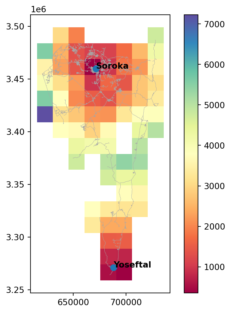
Figure 12.10 shows the results in the h_id column—the ID of the nearest hospital:
base = grid.plot(column='h_id', cmap='Set3', categorical=True, zorder=0)
net2.edges_to_gdf(G).plot(ax=base, linewidth=0.2, color='darkgrey', zorder=1)
geom.plot(ax=base, markersize=50, zorder=2)
for i in zip(locations, pnt):
    base.annotate(i[0].split(' ')[0], (i[1].x, i[1].y), ha='left', weight='bold');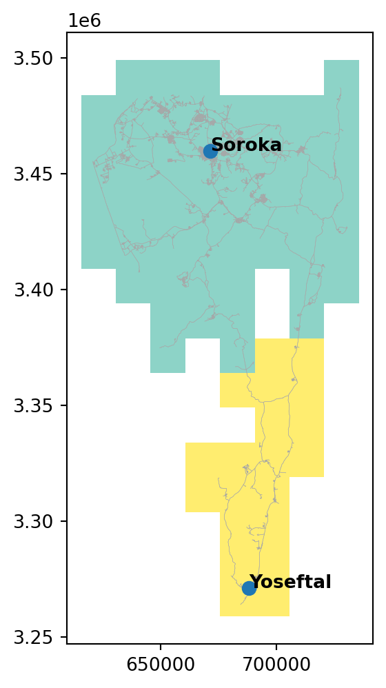
Exercises
Exercise 11-01
- Suppose that there was a new third hospital in the Negev, in Mitzpe Ramon
- What would the travel time and optimal allocation maps look like? (Figure 19.26)
Exercise 11-02
- Based on the Negev roads network (Figure 12.5), calculate a trave time matrix (Travel time matrix) between the following four locations:
locations = ['Eilat', 'Beer-Sheva', 'Neve Zohar', 'Nitzana']- Transform the matrix to a weighted spatial network, and draw a spatial plot of it, with node labels and edge labels (travel time in \(hr\)) (Figure 19.27)
Exercise 11-03
- Based on the Negev roads network (Figure 12.5), calculate a trave time matrix (Travel time matrix) between the following eight locations:
locations = ['Eilat', 'Ein-Gedi', 'Beer-Sheva', 'Neve Zohar', 'Mizpe Ramon', 'Nitzana', 'Arad', 'Sde Boker']- Transform the matrix to a weighted spatial network
- Use the
nx.approximation.traveling_salesman_problemfunction, as shown below, to solve the Traveling Salesman Problem, namely find the optimal route starting from'Beer-Sheva'and going through all eight nodes
nx.approximation.traveling_salesman_problem(G, weight='weight', source='Beer-Sheva')- Draw the spatial network of the eight locations, with the calculated optimal solution shown in red (Figure 19.28)