Introduction to Spatial Networks using Python
Preface
What are spatial networks?
Spatial networks are a specific case of networks, where nodes represent spatial locations, and edges represent connections between those locations. Phenomena that can be represented as spatial networks include, for example, road networks for car transport in a city (Figure 7.4), migration flow between continents (Figure 7.1), or existence of shared border between countries (Figure 19.9).

x and y coordinates. (Figure 1.1 from Barthelemy (2022))
A network-based representation of spatial phenomena and processes opens up the possibility for describing, visualizing, and analyzing the data using network analysis techniques, facilitating the ability to answer novel questions. For example, calculating an optimal route from one point to another along a road network (e.g., Figure 11.4) is only possible when representing the road data as a network data structure, and using network-specific algorithms for finding shortest paths.
What’s unique about spatial networks?
Working with networks also poses unique technical challenges, when compared to workflows with “traditional” spatial data. Traditional, or “ordinary”, spatial data can be thought of as collections of entities of the same type, whether vector features or raster pixels. Networks, however, are dual in nature, comprising entities of two types—nodes and edges. Accordingly, for example, a vector layer can be represented by a single table of features. The tabular representation of a network, on the other hand, comprises two interconnected tables.
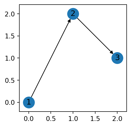
For example, Figure 2 depicts a minimal spatial network, which contains three nodes and two edges.
The nodes and edges of the network shown in Figure 2 can be represented using two tables, Table 1 for the nodes and Table 2 for the edges.
| id | geometry |
|---|---|
| 1 | POINT (0 0) |
| 2 | POINT (1 2) |
| 3 | POINT (2 1) |
| source | target | geometry |
|---|---|---|
| 1 | 2 | LINESTRING (0 0, 0 0) |
| 2 | 3 | LINESTRING (1 2, 1 2) |
Working with spatial networks therefore requires specialized computational tools, and a different kind of thinking, for even the simplest tasks. For example, spatial subsetting (i.e., “select by location”) of a vector layer is relatively straightforward: we retain those features whose geometry intersects with the area of interest (Figure 4.18). Subsetting a spatial network by location (Spatial subsetting), however, involves subsetting both the nodes and edges, while also keeping the network valid, e.g., if we retain a specific edge then we also must retain its nodes (Figure 6.14).
Why study spatial networks?
Study of spatial networks has numerous applications, for both basic research and practical applications. In basic research, spatial networks representation is essential for studying human travel behavior, accessibility, and public health. An obvious practical use of spatial network analysis is in routing applications, such as Google Maps (Figure 14.1). Other common practical use cases include service area calculations (Figure 12.10), optimal facility placement (i.e., “Location-Allocation”), and the Traveling Salesman Problem (Figure 19.28).
What are we going to learn?
This book teaches methods for working with spatial networks and analyzing them. We are going to cover the fundamental concepts and techniques of defining networks from various data sources, extracting descriptory information from networks, visualizing the networks, and answering questions related to the network arrangement. At first, we will mostly be working with a small road network, and few other simple networks. That way, we will be able to get familiar with network structures and their behavior, keeping track and understanding network processing workflows. We will introduce the specific considerations of defining road networks, and calculating optimal routes along road networks, such as road weighting profiles, and connectivity of new location to an existing network. We then demonstrate practical techniques related to routing, such as calculating shortest paths and evaluating accessibility. Subsequently, we are going to implement the tools we developed on real-world road networks, based on OpenStreetMap data. In the end of the course, we cover least cost path analysis on topographic rasters, which is another variant of spatial networks. There, we develop processing techniques from scratch, to demonstrate how our knowlege of spatial networks can be transfered to solve a novel type of analytical problem.
The material is demonstrated using the Python programming language, using packages networkx and osmnx, and others. We will extensively experiment with writing our own reusable functions for automation of network pre-processing, routing, and accessibility calculations.
Each book chapter consists of theory and practical examples, followed by exercises to do in class or at home.
By the end of the book, you will:
- become familiar with the network analysis approach to solving problems, i.e., be aware in which cases it can be useful and how can it be applied,
- understand what is happening “behind the scenes” when using off-the-shelf network analysis tools (e.g., network analysis tools in GIS software), and
- learn how to combine existing building blocks into your own functions of customized network analysis operations, to go beyond existing solutions and implement any novel analytical workflow you can think of
How is the book organized?
The book is split into three parts:
- Spatial data in Python—Brief overview of the Python language prerequisites: basic syntax, tables, arrays, vector layers, and rasters
- Spatial networks—covers the
networkxpackage for network analysis, and then moves on to spatial network analysis using bothnetworkxandosmnx, focusing on driving through road networks - Advanced topics—Covers select advanced topics, namely least cost path analysis using custom functions combined with
networkx, and consuming and building your own routing web services
Prerequisites
It is assumed that:
- You have a working Python environment where the third-party packages we are going to use (Software) are installed
- You are familiar with the basic Python syntax and data structures (such as
listanddict) (The Python language) - You are familiar with working with data in Python using
numpyandpandas(Data in Python) - You are familiar with working with spatial data in Python using
shapelyandgeopandas(Spatial data)
The first section of the book briefly goes over the material of 2-4. You should at least skim over these chapters to make sure that you understand the material and are ready for the main contents in parts 2 and 3 of the book (How is the book organized?).
Software
The software packages we are going to use in this book are listed in Table 3. The list includes the Python software itself, and several Python packages.
To reproduce the code examples in this book, you need to install lxml, scipy, matplotlib, osmnx, rasterio, fastapi, and geopy. All other required packages are their dependencies, and installed automatically.
Datasets
The code examples in the book rely on several sample data files, which are summarized in Table 4. To reproduce the examples, you need to download the data files from the following link:
Then, extract the files and place them into a directory named data.
Some of the code examples export the results to files, into a directory named output. Create an empty directory named output to reproduce these code sections.
| File(s) | Description | Source | Accessed |
|---|---|---|---|
dem.tif |
Digital elevation model | https://www.earthdata.nasa.gov/data/catalog/lpcloud-srtmgl1-003 | 2025 |
europe.gpkg |
Europe countries | https://www.naturalearthdata.com/downloads/110m-cultural-vectors | 2023 |
gas-stations.geojson |
Minimal road network | https://data.gov.il/dataset/gas-stations-br7 | 2023 |
mapbox_response.json |
Mapbox Directions API response | https://docs.mapbox.com/api/navigation/directions/ | 2025 |
ne_110m_admin_0_countries.shp |
World countries | https://www.naturalearthdata.com/downloads/110m-cultural-vectors | 2023 |
roads.xml |
Minimal road network | https://docs.pgrouting.org/latest/en/sampledata.html | 2023 |
Output files
As part of the code examples in the book, we are going to export data into new files. These files are going to be created in a directory named output. Some of the output files will be used as inputs in other code examples in the book. To be sure that you can run the code examples in any given chapter, you can also download the output files from the following link:
Then, extract the files and place them into a directory named output.
The net2 module
Throughtout the book, we are going to develop functions for network processing and analysis, which we are going repeatedly use in various chapters and code examples. To avoid code duplication, the functions will be stored in a module (Custom modules) named net2.py.
The net2.py file should be placed in the directory where the data (Datasets) and output (Output files) directories are.
Directory tree
Once you have downloaded data.zip, output.zip, and net2.py, and extracted the former two into the respective directories, you should have the following directory structure:
┌── data
│   ├── dem.tif
│   ├── europe.gpkg
│   ├── gas-stations.geojson
│   ├── mapbox_response.json
│   ├── ne_110m_admin_0_countries.cpg
│   ├── ne_110m_admin_0_countries.dbf
│   ├── ne_110m_admin_0_countries.prj
│   ├── ne_110m_admin_0_countries.shp
│   ├── ne_110m_admin_0_countries.shx
│   └── roads.xml
├── output
│   ├── beer-sheva_edges.gpkg
│   ├── beer-sheva.xml
│   ├── continents1.xml
│   ├── continents2.xml
│   ├── europe_borders.csv
│   ├── hospitals.csv
│   ├── hospitals.gpkg
│   ├── negev.xml
│   └── roads2.xml
└── net2.py

3 directories, 20 files
In this working directory, you can place and run code examples from the book, assuming that you have a working Python environment where the required packages are installed (Software).
Resources
Overview
This section lists recommended resourses about spatial networks in Python.
Courses
Python packages
Papers
- Boeing, G. (2025). Modeling and Analyzing Urban Networks and Amenities with OSMnx. Geographical Analysis 57 (4), 567-577. doi:10.1111/gean.70009
- Boeing, G. (2025). Topological Graph Simplification Solutions to the Street Intersection Miscount Problem. Transactions in GIS 29 (3), e70037. doi:10.1111/tgis.70037
- Boeing, G. (2021). Street Network Models and Indicators for Every Urban Area in the World. Geographical Analysis 54 (3), 519-535. doi:10.1111/gean.12281
- Boeing, G. (2020). The Right Tools for the Job: The Case for Spatial Science Tool-Building. Transactions in GIS 24 (5), 1299-1314. doi:10.1111/tgis.12678
- Boeing, G. (2020). Planarity and Street Network Representation in Urban Form Analysis. Environment and Planning B: Urban Analytics and City Science 47 (5), 855-869. doi:10.1177/2399808318802941
System information
Python version used when rendering the book is:
3.12.3 (main, Jan 22 2026, 20:57:42) [GCC 13.3.0]Package versions are:
numpy==2.1.1
pandas==3.0.1
shapely==2.1.2
geopy==2.4.1
pyproj==3.7.0
geopandas==1.1.2
matplotlib==3.10.7
rasterio==1.5.0
networkx==3.3
osmnx==2.0.2
fastapi==0.115.12
Hostname is:
dell14