Last updated: 2026-03-04 01:46:42Raster least cost paths
Introduction
In the last several chapters, we introduced the concept of spatial networks through a specific type of a network: a road network. Though a very common one, road networks are not the only type of a spatial network. In this chapter, we are going to deal with a different type of a spatial network: a landscape defined using a Digital Elevation Model (DEM). As we go through this chapter, you will not only become familiar with another type of network; you will also see how the general principles of spatial networks—nodes locations, edges geometries, weights, directions, routing, etc.—are not specific to roads, but can be applied to a very different type of network, mostly using the same data structures and functions you are familiar with.
In this chapter, we will go through two examples of calculating shortest paths over topographic terrain:
- a minimal example of a synthetic digital elevation model (Figure 13.3)
- a realistic example of the Grand Canyon terrain (Figure 13.7)
We will go through the following steps:
- Developing a function for estimating weights of walking on terrain (Tobler’s hiking function)
- Minimal example
- Preparing sample raster (Sample data (1))
- Creating raster nodes (Creating raster nodes (1))
- Creating raster edges (Creating raster edges (1))
- Calculating a least cost path (Least cost path (1))
- Realistic DEM of the Grand Canyon
- Preparing sample raster (Sample data 2)
- Creating raster nodes (Creating raster nodes (2))
- Creating raster edges (Creating raster edges (2))
- Calculating a least cost path (Least cost paths (2))
Packages
import math
import matplotlib.pyplot as plt
import numpy as np
import shapely
import networkx as nx
import net2
import rasterio
import rasterio.plot
Tobler’s hiking function
In this chapter, we are going to learn how to calculate optimal walking routes across a landscape defined by a digital elevation model. Unlike a road network, where travel time is primarily determined by maximum driving speed (Calculating travel times), when modeling the landscape we primarily consider the elevation change, or slope. To do that, we need to define the association between slope and walking speed.
Tobler’s hiking function is a commonly used formula estimating walking speed as function of slope. Tobler’s hiking function is defined as follows (Equation 13.1):
\[ speed (km/hr) = 6 \times {\rm e}^{-3.5 | \frac{dh}{dx} + 0.05|} \tag{13.1}\]
where \(dh\) is the elevation difference, and \(dx\) is the distance.
Here is how we can translate Tobler’s hiking function into a Python function named walking_speed_km_hr. The function accepts the elevation difference and a distance ratio dh_by_dx, and returns the walking speed in \(km/hr\):
def walking_speed_km_hr(dh_by_dx):
    return 6*2.718**(-3.5*abs(dh_by_dx+0.05))
Let’s demonstrate how the function works. For example, the estimated walking speed on flat terrain (i.e., \(dh/dx=0\)) is ~5.04 \(km/hr\):
walking_speed_km_hr(0) ## Flat terrain5.036833515858116The maximum walking speed of 6.00 \(km/hr\) is attained in a gradient of \(dh/dx=-0.05\), i.e., a slope of \(-2.8624 \degree\), such as when walking 30 \(m\) on such a sloped surface that elevation change is -1.5 \(m\):
walking_speed_km_hr(-1.5/30) ## Optimal gradient (slope -2.8624 deg.)6.0Sometimes we want to define the slope using an angle, rather than elevation and distance (\(dh/dx\)). In such case, we can translate slope \(\theta\) to \(dh/dx\) using Equation 13.2:
\[ \frac{dh}{dx} = \tan{\theta (radians)} \tag{13.2}\]
For example, suppose that we want to calculate the walking speed over the steep slope of \(50 \degree\). We can apply Equation 13.2, using np.tan and also converting from degrees to radians–which np.tan expects—using np.deg2rad:
x = np.tan(np.deg2rad(50))
xnp.float64(1.19175359259421)The resulting \(\frac{dh}{dx}\) value can then be passed to our implementation of Equation 13.1—walking_speed_km_hr:
walking_speed_km_hr(x) ## Very steep gradientnp.float64(0.07777560333824717)Let’s demonstarate the relationship between slopes and walking speeds by plotting the walking_speed_km_hr function. To do that, we can first create an array of 500 slopes, at equal intervals, covering the range between \(-60 \degree\) and \(50 \degree\), named dh_by_dx:
slope = np.linspace(-60, 50, 500)
dh_by_dx = np.tan(np.deg2rad(slope))
dh_by_dx[:5]
array([-1.73205081, -1.71676293, -1.70167569, -1.68678472, -1.67208578])The walking_speed_km_hr function can be applied on the array, to get the corresponding array of walking speeds:
speed_km_hr = walking_speed_km_hr(dh_by_dx)
speed_km_hr[:5]
array([0.01665895, 0.01757451, 0.01852737, 0.01951849, 0.02054881])Figure 13.1 plots the array of walking speeds (speed_km_hr, on the y-axis) for each of the slopes (slope, on the x-axis):
plt.axvline(x=0, color='grey', linewidth=1, linestyle='--')
plt.axhline(y=5, color='grey', linewidth=1, linestyle='--')
plt.plot(slope, speed_km_hr, color='red')
plt.xlabel('Slope ($\\degree$)')
plt.ylabel('Walking speed ($km/hr$)')
plt.ylim(ymin=0);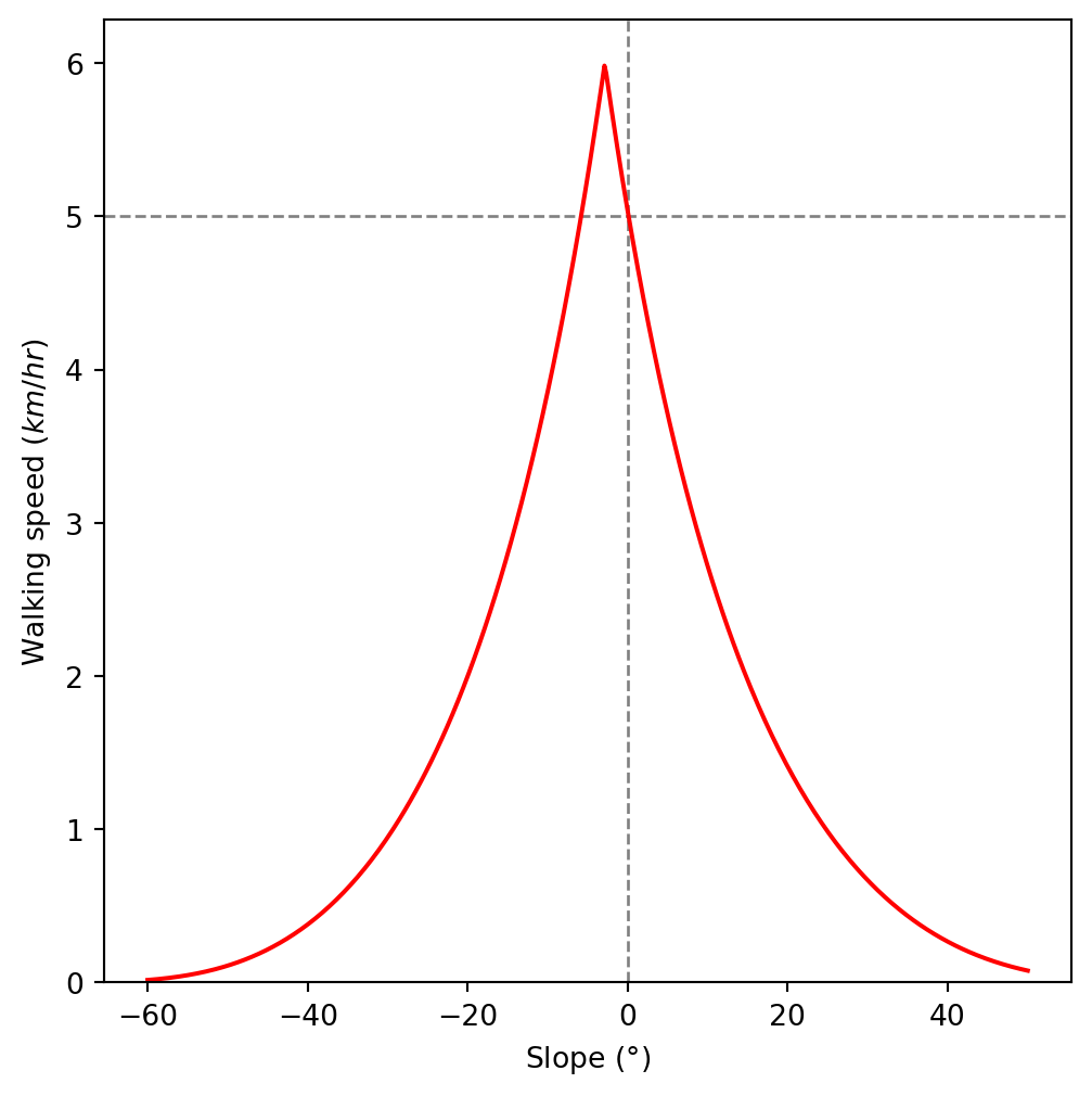
As we can see in Figure 13.1, the fastest walking speed is obtained in a slightly downward slope.
Our network weights are going to be expressed in travel times, rather than speeds. Therefore, we will write a wrapper function named walking_time_sec, which calculates travel time in \(sec\). Note that walking_time_sec requires dh and dx as separate arguments, since the travel time is calculated as the quotient of walked distance dx and speed. Assuming that dx and dh are in \(m\), using Equation 7.1, we get:
def walking_time_sec(dh, dx):
    speed = walking_speed_km_hr(dh / dx)
    time = (dx / speed) * 3.6
    return time
Here are is an example of applying the function:
walking_time_sec(-1.5, 30)18.0Again, we can plot the function to see what the relationship looks like. First, we create an array of slopes, this time between \(-40 \degree\) and \(40 \degree\):
slope = np.linspace(-40, 40, 500)
dh_by_dx = np.tan(np.deg2rad(slope))
dh_by_dx[:5]
array([-0.83909963, -0.83434254, -0.82960761, -0.82489461, -0.82020332])Assuming that \(dx\) is 1 \(m\), then \(\frac{dh}{dx}=\frac{dh}{1}=dh\). So we can pass \(\frac{dh}{dx}\) for dh, and 1 for dx. The result is an array of the time it takes to cover 1 \(m\) of terrain, for each of the slopes, in \(sec\):
time = walking_time_sec(dh_by_dx, 1)
time[:5]
array([9.49472826, 9.33796763, 9.18450742, 9.03426256, 8.88715057])Figure 13.2 shows the resulting relation:
plt.axvline(x=0, color='grey', linewidth=1, linestyle='--')
plt.plot(slope, time, color='red')
plt.xlabel('Slope ($\\degree$)')
plt.ylabel('Walking pace ($sec/m$)')
plt.ylim(ymin=0);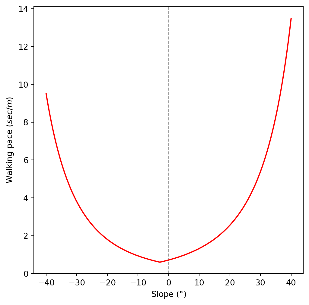
You can see, again, that the optimal pace is obtained in a slightly downward slope.
Sample data (1)
In our first example of calculating least cost paths, we will use a small synthetic array, representing a “made up” elevation model. This is a \(5 \times 5\) DEM, with two possible elevation values of 0 and 2:
r = [
  [0, 0, 0, 0, 0],
  [2, 2, 2, 2, 0],
  [0, 0, 2, 0, 0],
  [0, 2, 2, 2, 0],
  [0, 0, 0, 0, 0]
]
r = np.array(r)
r
array([[0, 0, 0, 0, 0],
[2, 2, 2, 2, 0],
[0, 0, 2, 0, 0],
[0, 2, 2, 2, 0],
[0, 0, 0, 0, 0]])Then, we prepare an arbitrary transformation matrix. The transformation matrix associates array indices with spatial coordinates, which is the differentiating feature between an ordinary array and a spatial raster. In this case, we arbitrarily set the origin of the raster to be (0,0), and the resolution to be (1,1):
transform = rasterio.transform.from_origin(
    west=0,
    north=0,
    xsize=1,
    ysize=1
)
transform
Affine(1.0, 0.0, 0.0,
0.0, -1.0, 0.0)We will also prepare a transformer function—named transformer—based on the transform object, to actually calculate the pixel coordinates:
transformer = rasterio.transform.AffineTransformer(transform)
transformer<AffineTransformer>The transformer object has an .xy method which can be used to calculate the coordinates:
transformer.xy<bound method TransformerBase.xy of <AffineTransformer>>For example, here are the coordintes of the pixel in the top-left corner (row 0, column 0):
transformer.xy(0, 0)(np.float64(0.5), np.float64(-0.5))If we need the coordinates to be in a plain numeric list, rather than a list of numpy arrays, here is an expanded expression:
[float(i) for i in transformer.xy(0, 0)][0.5, -0.5]The minimal synthetic digital elevation model is shown in Figure 13.3. Since we pass the transform object to the plotting function, you can see the actual pixel coordinates on the x-axis and the y-axis:
rasterio.plot.show(r, transform=transform);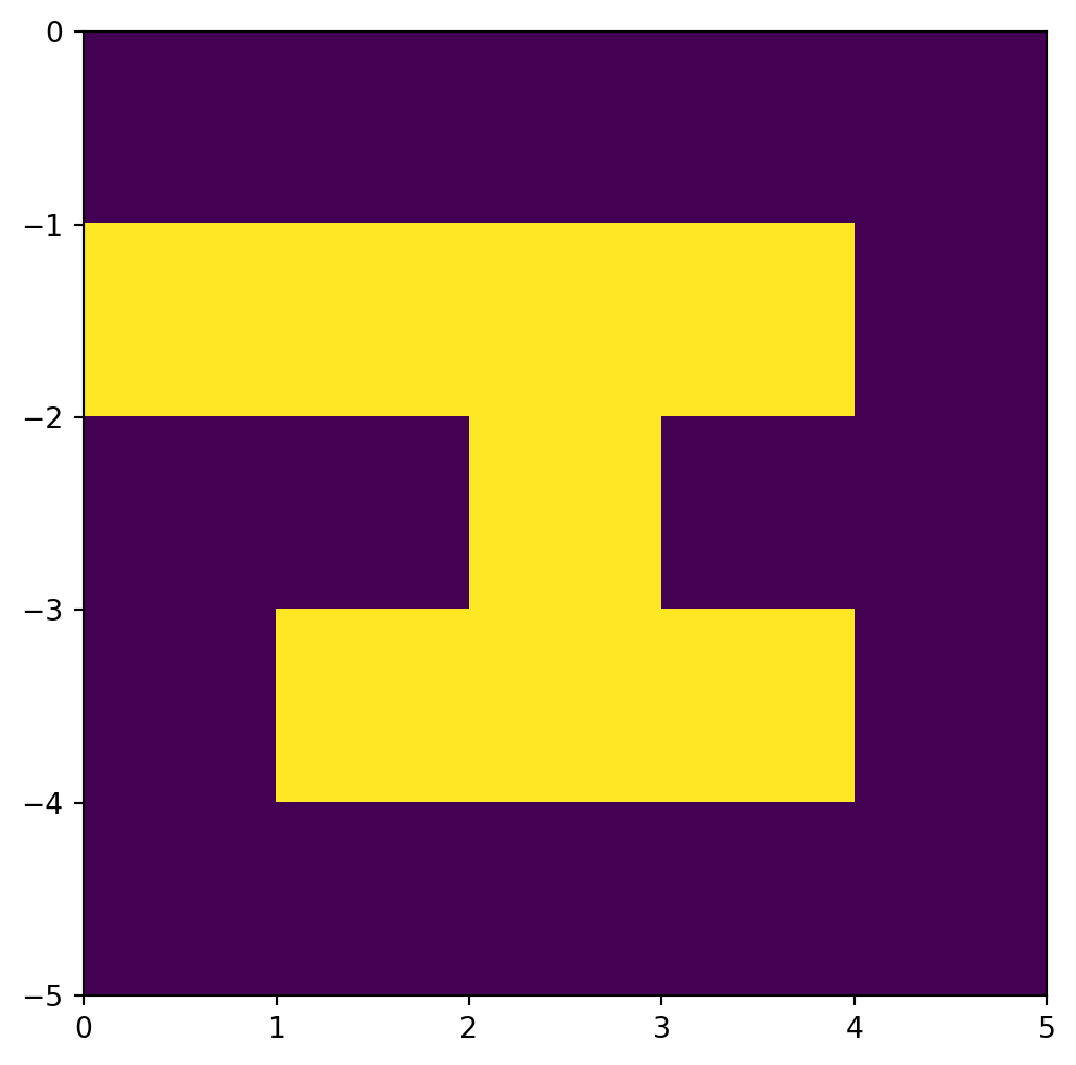
Creating raster nodes (1)
To calculate least cost paths, we need to prepare the spatial network representing the DEM. In the network:
- Nodes represent raster cells
- Edges represent possible steps a person can take from one cell to any of the 8 neighboring cells
First, we initialize an empty directed network named G:
G = nx.Graph()
G = G.to_directed()
G
<networkx.classes.digraph.DiGraph at 0x7bcf5bb25bb0>Then, for each row i and each column j of the raster, we:
- Initialize a new node
(i,j) - Calcualate the spatial coordinates of the corresponding pixel, and assign them to the node properties
xandy - Extract the raster value (i.e., elevation) of the corresponding pixel, and assign it to the node property
z
for row in range(r.shape[0]):
    for col in range(r.shape[1]):
        G.add_node((row, col))
        coords = [float(i) for i in transformer.xy(row, col)]
        G.nodes[(row, col)]['geometry'] = shapely.Point(coords)
        G.nodes[(row, col)]['z'] = r[row, col]
By the end of the loop, the network G contains all possible edges between neighboring raster cells:
G.number_of_nodes()25For example, here is the node representing the top-left raster cell (row 0, column 0):
G.nodes[0,0]{'geometry': <POINT (0.5 -0.5)>, 'z': np.int64(0)}and here is the node representing the cell directly beneath it (row 1, column 0):
G.nodes[1,0]{'geometry': <POINT (0.5 -1.5)>, 'z': np.int64(2)}At this point, we have a spatial network with just the nodes representing the raster cells (Figure 13.4):
nx.draw(G, with_labels=True, pos=net2.pos(G))
Creating raster edges (1)
Now we move on to calculating the raster edges. First, let’s define a variable named res with the raster resolution, which we can extract from the transformation matrix transform. The resolution of the minimal DEM is 1 (Figure 13.3):
res = transform[0]
res1.0Next, we define a function named calculate_time, which accepts the array r, origin and destination nodes (orig and dest, respectively), and the resolution res, and returns the walking time between the nodes. The calculate_time function essentially “wraps” the walking_time_sec function defined above (see Tobler’s hiking function). However, the walking_time_sec function requires dx and dh, which are derived from r, orig, dest, and res, as follows:
dxis either equal to \(res\) in a vertical or horizontal movement, or to \(\sqrt{2} \times res\) in a diagonal movementdhis equal to the elevation difference of the two raster cellsr[dest]andr[orig]
def calculate_time(r, orig, dest, res):
    if orig[0] == dest[0] or orig[1] == dest[1]:
        dx = res
    else:
        dx = math.sqrt(2) * res
    elev0 = r[orig]
    elev1 = r[dest]
    dh = elev1 - elev0
    time = walking_time_sec(dh, dx)
    time = float(time)
    time = round(time, 4)
    return time
Note
Note that the calculate_time function only makes sense for adjacent orig and dest.
For example, considering the top-left raster cell orig and the cell directly beneath it dest:
orig = (0, 0)
dest = (1, 0)
Here is the walking time from orig to dest:
calculate_time(r, orig, dest, res)783.2332Other than 'time', we want each edge to have a 'geometry' attribute. To calculate the geometry, we define a function named calculate_line as follows:
def calculate_line(orig, dest, transformer):
    pnt0 = [float(i) for i in transformer.xy(orig[0], orig[1])]
    pnt1 = [float(i) for i in transformer.xy(dest[0], dest[1])]
    geom = shapely.LineString([pnt0, pnt1])
    return geom
Now we can move on to calculating the network edges. Similarly to the node calculation (Creating raster nodes (1)), we go over each raster row (row) and column (col) combination, i.e., each cell (row,col). However, within each (row,col), we have two more for loops, to go over each row_offset and col_offset, each of them taking one of the values [-1,0,1]. The internal loops represent all 9 possible directions from the focal cell to its neighbors or self. Two edge cases are skipped:
- The destination cell is the same as the origin
- The destination cell is supposedly outside of the raster extent
and then the edge (orig, dest), along with the calculated 'time' and 'geometry' attributes, is being added to the network G:
for row in range(r.shape[0]):
    for col in range(r.shape[1]):
        orig = (row, col)
        for row_offset in [-1, 0, 1]:
            for col_offset in [-1, 0, 1]:
                dest = row + row_offset, col + col_offset
                # Destination is same pixel
                if row_offset == 0 and col_offset == 0:
                    continue
                # Destination is outside of raster
                if dest[0] < 0 or dest[0] >= r.shape[0] or dest[1] < 0 or dest[1] >= r.shape[1]:
                    continue
                G.add_edge(orig, dest)
                G.edges[orig, dest]['time'] = calculate_time(r, orig, dest, res)
                G.edges[orig, dest]['geometry'] = calculate_line(orig, dest, transformer)
By the end of the loop, the network G contains all possible edges between neighboring raster cells:
G.number_of_edges()144For example, here is the edge going from the top-left cell 0,0 to the cell directly beneath it (1,0):
G.edges[(0,0), (1,0)]{'time': 783.2332, 'geometry': <LINESTRING (0.5 -0.5, 0.5 -1.5)>}this is an example of a vertical edge (of length 1), which can be demonstrated by drawing its geometry:
G.edges[(0,0), (1,0)]['geometry']
Here is an example of a diagonal edge:
G.edges[(0,0), (1,1)]{'time': 142.5887, 'geometry': <LINESTRING (0.5 -0.5, 1.5 -1.5)>}as demonstrated by drawing the geometry:
G.edges[(0,0), (1,1)]['geometry']
Figure 13.5 shows the network G, now also with weighted edges:
nx.draw(G, with_labels=True, pos=net2.pos(G), connectionstyle='arc3,rad=0.1')
edge_labels = nx.get_edge_attributes(G, 'time')
nx.draw_networkx_edge_labels(G, net2.pos(G), edge_labels, connectionstyle='arc3,rad=0.1', font_size=5);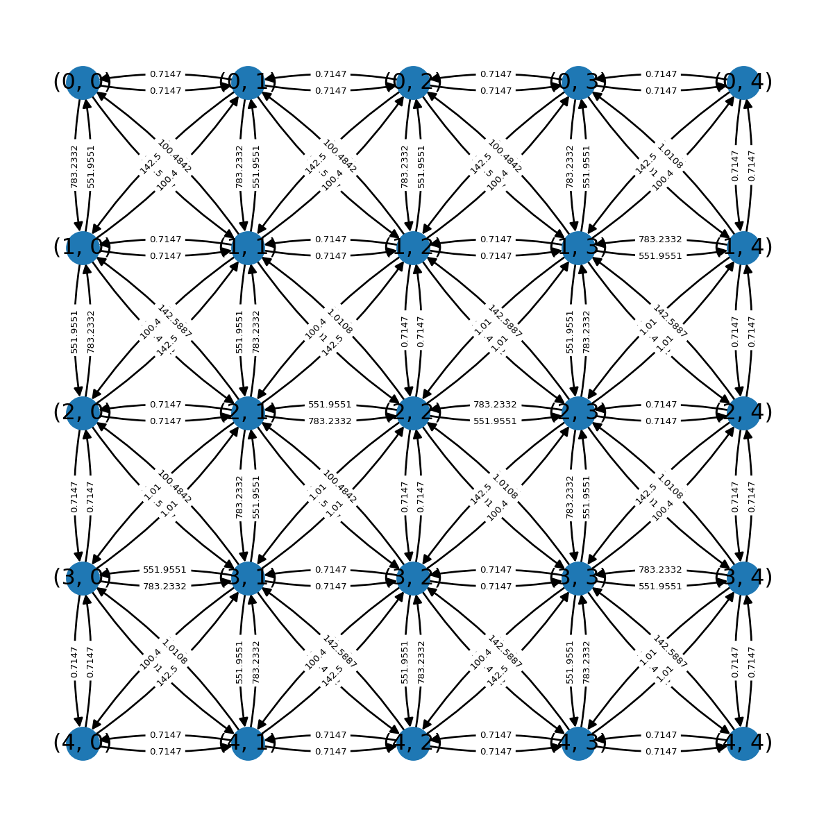
The network G representing walking routes through the raster topography is now ready, and we can move on to demonstrate a least cost path calculation (Least cost path (1)).
Least cost path (1)
Finally, we can demonstrate a calculation of an optimal walking route through the terrain, also known as a least cost path. For example, let’s define the origin cell as the top-left corner of the raster:
orig = (0, 0)
orig
(0, 0)and the destination cell as the cell three “steps” beneath it:
dest = (3, 0)
dest
(3, 0)We can pass the network, origin, and destination, to the net2.route1 function (Basic routing function), while specifying 'time' as the weight being minimized. As a result, we get the route and total travel time:
route = net2.route1(G, orig, dest, 'time')
route
{'route': [(0, 0),
(0, 1),
(0, 2),
(0, 3),
(1, 4),
(2, 4),
(3, 4),
(4, 3),
(4, 2),
(4, 1),
(3, 0)],
'weight': 8.0353}Using net2.route_to_gdf (Route to GeoDataFrame), we can transform the route to a GeoDataFrame:
line = net2.route_to_gdf(G, route['route'])
line| from | to | geometry | |
|---|---|---|---|
| 0 | (0, 0) | (0, 1) | LINESTRING (0.5 -0.5, 1.5 -0.5) |
| 1 | (0, 1) | (0, 2) | LINESTRING (1.5 -0.5, 2.5 -0.5) |
| 2 | (0, 2) | (0, 3) | LINESTRING (2.5 -0.5, 3.5 -0.5) |
| ... | ... | ... | ... |
| 7 | (4, 3) | (4, 2) | LINESTRING (3.5 -4.5, 2.5 -4.5) |
| 8 | (4, 2) | (4, 1) | LINESTRING (2.5 -4.5, 1.5 -4.5) |
| 9 | (4, 1) | (3, 0) | LINESTRING (1.5 -4.5, 0.5 -3.5) |
10 rows × 3 columns
Figure 13.6 shows the origin and destination points and the calculated route, along with the DEM in the background:
fig, ax = plt.subplots()
rasterio.plot.show(r, transform=transform, ax=ax)
line.plot(ax=ax, edgecolor='red')
plt.plot(*transformer.xy(*orig), 'wx', markersize=12)
plt.plot(*transformer.xy(*dest), 'wx', markersize=12);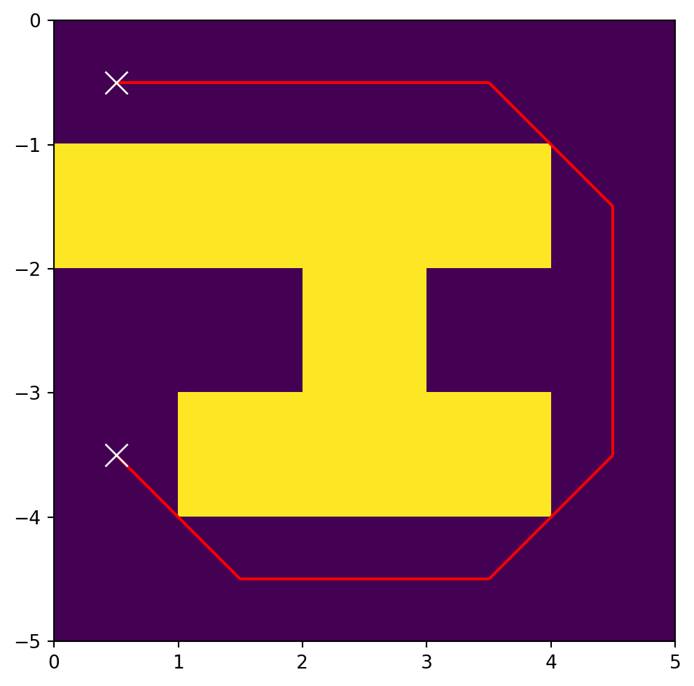
Sample data 2
In our second least cost path example in this chapter, we are going to use a realistic DEM example: a DEM of a \(7.5 \times 7.5\) \(km^2\) extent over the Grand Canyon. The DEM is stored in a GeoTIFF file named dem.tif. To use the data in Python, we need to create a file connection, using rasterio.open:
src = rasterio.open('data/dem.tif')Figure 13.7 shows the DEM:
rasterio.plot.show(src);
Let’s also read the array with the raster values:
r = src.read(1)This is a larger DEM, with \(250 \times 250\) pixels:
r.shape(250, 250)and realistic elevation values, in \(m\) above sea level:
r[:3, :3]array([[1703.5546, 1699.9779, 1691.0651],
[1704.1259, 1695.7571, 1686.433 ],
[1699.1866, 1687.0507, 1672.4417]], dtype=float32)As can be observed in the raster file metadata, the raster has a built-in transformation matrix and is associated with a CRS (EPSG:32612):
src.meta{'driver': 'GTiff',
'dtype': 'float32',
'nodata': None,
'width': 250,
'height': 250,
'count': 1,
'crs': CRS.from_wkt('PROJCS["WGS 84 / UTM zone 12N",GEOGCS["WGS 84",DATUM["WGS_1984",SPHEROID["WGS 84",6378137,298.257223563,AUTHORITY["EPSG","7030"]],AUTHORITY["EPSG","6326"]],PRIMEM["Greenwich",0,AUTHORITY["EPSG","8901"]],UNIT["degree",0.0174532925199433,AUTHORITY["EPSG","9122"]],AUTHORITY["EPSG","4326"]],PROJECTION["Transverse_Mercator"],PARAMETER["latitude_of_origin",0],PARAMETER["central_meridian",-111],PARAMETER["scale_factor",0.9996],PARAMETER["false_easting",500000],PARAMETER["false_northing",0],UNIT["metre",1,AUTHORITY["EPSG","9001"]],AXIS["Easting",EAST],AXIS["Northing",NORTH],AUTHORITY["EPSG","32612"]]'),
'transform': Affine(30.0, 0.0, 340150.5054945286,
0.0, -30.0, 4025687.7291128924)}Creating raster nodes (2)
Next we create the network nodes, using essentialy the same code as for the minimal DEM (sec-creating-raster-nodes-1). The only difference is that the transform now comes from the raster metadata, and is a realistic rather than an arbitrary one:
transform = src.transform
transform
Affine(30.0, 0.0, 340150.5054945286,
0.0, -30.0, 4025687.7291128924)transformer = rasterio.transform.AffineTransformer(transform)
transformer<AffineTransformer>G = nx.Graph()
G = G.to_directed()
G<networkx.classes.digraph.DiGraph at 0x7bcf60a9b140>for row in range(r.shape[0]):
for col in range(r.shape[1]):
G.add_node((row, col))
coords = [float(i) for i in transformer.xy(row, col)]
G.nodes[(row, col)]['geometry'] = shapely.Point(coords)
G.nodes[(row, col)]['z'] = r[row, col]Here is an example of a node representing the top-left raster corner:
G.nodes[0,0]{'geometry': <POINT (340165.505 4025672.729)>, 'z': np.float32(1703.5546)}Creating raster edges (2)
Next we add the network edges, using exactly the same code as in the minimal example (Creating raster edges (1)):
res = src.transform[0]
res30.0for row in range(r.shape[0]):
for col in range(r.shape[1]):
orig = (row, col)
for row_offset in [-1, 0, 1]:
for col_offset in [-1, 0, 1]:
dest = row + row_offset, col + col_offset
# Destination is same pixel
if row_offset == 0 and col_offset == 0:
continue
# Destination is outside of raster
if dest[0] < 0 or dest[0] >= r.shape[0] or dest[1] < 0 or dest[1] >= r.shape[1]:
continue
G.add_edge(orig, dest)
G.edges[orig, dest]['time'] = calculate_time(r, orig, dest, res)
G.edges[orig, dest]['geometry'] = calculate_line(orig, dest, transformer)Here is an example of an edge:
G.edges[(0,0),(1,1)]{'time': 40.6564,
'geometry': <LINESTRING (340165.505 4025672.729, 340195.505 4025642.729)>}Least cost paths (2)
Now that the network is ready, we can demonstrate a least cost path calculation. We will take two points, chosen in advance so that they are within the Grand Canyon (Figure 13.8):
pnt0 = shapely.Point(341860, 4019850)
pnt1 = shapely.Point(345945, 4024014)
Unlike in the minimal example, here the origin (pnt0) and destination (pnt1) points are represented using spatial coordinates (in EPSG:32612). To use the net2.route1 function, we need to “translate” those point coordinates to the IDs of the nearest nodes, orig and dest, respectively. We do that using the net2.nearest_node function (Nearest node):
orig = net2.nearest_node(G, pnt0)[0]
dest = net2.nearest_node(G, pnt1)[0]
orig, dest
((194, 56), (55, 193))Now we can calculate the optimal route in terms of 'time':
route = net2.route1(G, orig, dest, 'time')
route['route'][:5]
[(194, 56), (193, 57), (192, 58), (191, 58), (190, 58)]Here is the total travel time in hours:
route['weight'] / (60 * 60)2.0941008611111123Let’s transform the route to a GeoDataFrame to display it:
line = net2.route_to_gdf(G, route['route'])
line| from | to | geometry | |
|---|---|---|---|
| 0 | (194, 56) | (193, 57) | LINESTRING (341845.505 4019852.... |
| 1 | (193, 57) | (192, 58) | LINESTRING (341875.505 4019882.... |
| 2 | (192, 58) | (191, 58) | LINESTRING (341905.505 4019912.... |
| ... | ... | ... | ... |
| 265 | (57, 193) | (57, 194) | LINESTRING (345955.505 4023962.... |
| 266 | (57, 194) | (56, 194) | LINESTRING (345985.505 4023962.... |
| 267 | (56, 194) | (55, 193) | LINESTRING (345985.505 4023992.... |
268 rows × 3 columns
Figure 13.8 shows the calculated route. As can be expected, the optimal walking route, in terms of topography, follows the Colorado River:
fig, ax = plt.subplots()
rasterio.plot.show(r, transform=src.transform, ax=ax)
line.plot(ax=ax, edgecolor='red')
plt.plot(pnt0.x, pnt0.y, 'wx', markersize=8)
plt.plot(pnt1.x, pnt1.y, 'wx', markersize=8);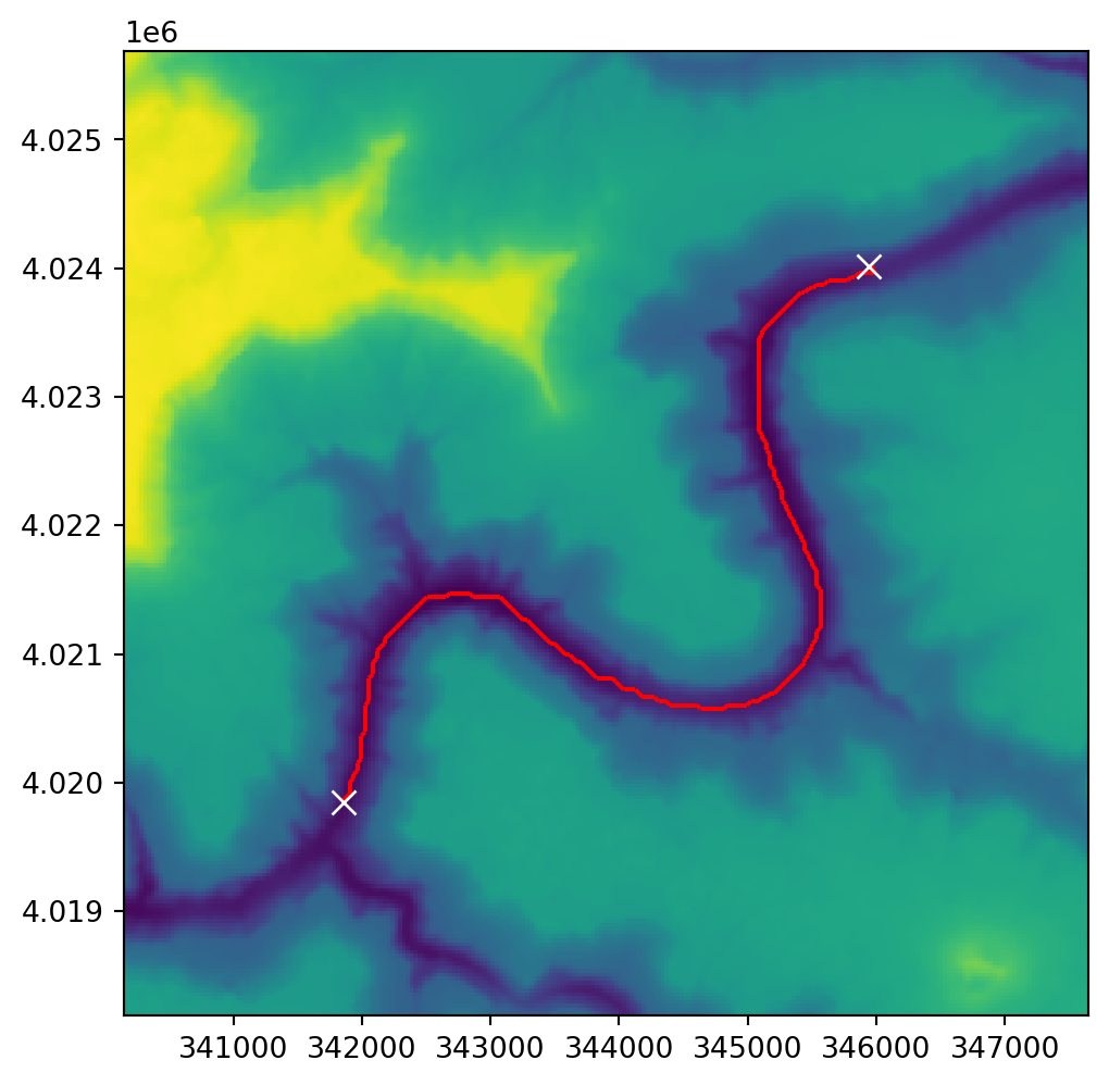
Exercises
Exercise 12-01
- Using the Grand Canyon DEM network (Figure 13.8), calculate and plot:
- Optimal route from the top-left to bottom-right corner
- Optimal route from the bottom-left to top-right corner (Figure 19.29)
Exercise 12-02
- Use the code section below to read a resampled lower resolution version of the Grand Canyon DEM (
r), and the corresponding updated transform matrix (new_transform) (this is to make the subsequent calculation faster) - Calculate and plot a raster of travel times from one specific point (of your choice), to all raster pixels, i.e., an accessibility map (Figure 19.30)
factor = 0.5
src = rasterio.open('data/dem.tif')
r = src.read(1,
    out_shape=(
        int(src.height * factor),
        int(src.width * factor)
    ),
    resampling=rasterio.enums.Resampling.average
)
new_transform = src.transform * src.transform.scale(
    (src.width / r.shape[-1]),
    (src.height / r.shape[-2])
)
Exercise 12-03
- Repeat Exercise 10-01, but this time create and plot a raster—instead of a polygonal layer—of travel times (Figure 19.31)