OpenStreetMap and osmnx

Last updated: 2026-03-04 01:42:40

Introduction

In this chapter, we demonstrate data preparation and routing workflows using realistic road networks from OpenStreetMap (OSM).

• First, we introduce OSM (What is OpenStreetMap (OSM)?)

• Then, we show how to load road network data from OSM into the Python environment (Loading OSM data)

• To make the network useable for routing, we go through several pre-processing steps (Filtering components, Imputing travel times, MultiDiGraph to DiGraph, Standardizing the network, Deleting unnecessary attributes, Filling edge geometries, Projecting geometries)

• Once the network is ready, we demonstrate routing functionality on it (Routing (OSM))

• Finally, prepare a regular grid covering the network (Customized regular grid), which we can use for accessibility calculations

Packages

import pandas as pd
import matplotlib.pyplot as plt
import shapely
import geopandas as gpd
import networkx as nx
import osmnx as ox
import pyproj
import net2

What is OpenStreetMap (OSM)?

OpenStreetMap (OSM) is a free global database of geographic data (Figure 11.1). The data in OSM are contributed and maintained by volunteers, similarly to Wikipedia. Thanks to the extensive coverage and availability, OSM data is the main data source for mapping, in general, and for network analysis and routing applications, in particular.

Figure 11.1: OpenStreetMap homepage

OSM provides several standard background layers, regularly updated, on the OSM homepage (Figure 11.1), and also as services to be used in any custom map. Moreover, importantly, OSM provides the raw data that is behind the maps, i.e., the point, line, and polygon coordinates, and attributes, comprising the features you see on the map. Attributes, known as “tags” in OSM terminology, can be used to differentiate features of particular type. For example, for routing we are typically interested only the road features, along with their type and/or speed limit information.

OSM Road types

In OSM, The key highway=* is used for identifying various kinds of roads, streets, or paths. Only some of the line segments marked with the highway=* tag are suitable for driving routing appications. Here are the most important highway values relevant for driving:

• "living_street"
• "motorway"
• "motorway_link"
• "primary"
• "primary_link"
• "residential"
• "secondary"
• "secondary_link"
• "tertiary"
• "tertiary_link"
• "trunk"
• "trunk_link"
• "unclassified"

Segments marked with other values, such as "path", "pedestrian", and "track", are unsuitable for driving.

What is osmnx

osmnx (Boeing 2017) is a Python package with functions to download, process, and analyze street network data from OSM. Raw OSM data require pre-processing to be suitable for network analysis. osmnx does two important pre-processing tasks (Boeing 2025) after downloding OSM data:

• Simplification—discarding nodes that do not comprise true intersections
• Consolidation—merging multiple nodes, comprising complex intersections (e.g., traffic circles), into one

Loading OSM data

The osmnx package provides several functions to download network data from OSM. These functions differ in the way that the area of interest is specified. For example:

• ox.graph_from_bbox—A (lon0,lat0,lon1,lat1) bounding box
• ox.graph_from_place—A place name str
• ox.graph_from_point—A (lat,lon) point and distance in \(m\)
• ox.graph_from_polygon—A shapely polygon

Note

The pyosrm package provides an alternative method to obtain street networks from OSM that is more suitable for large areas.

For the examples in this chapter, we are going to download the Beer-Sheva road network using ox.graph_from_bbox:

b = [34.75, 31.2, 34.83, 31.31]
b

[34.75, 31.2, 34.83, 31.31]

Using ox.graph_from_bbox, the following expression downloads OSM road data for the specified extent b, and transforms it to the networkx object named G. Note that we are using network_type='drive', which considers only routable roads for cars when creating the network:

G = ox.graph_from_bbox(b, network_type='drive', truncate_by_edge=True)
G

<networkx.classes.multidigraph.MultiDiGraph at 0x74cad33cd910>

In the following sections, we are going to further process and prepare the object G. Then, after it is ready, we will demonstrate routing calculations in a realistic road network (Routing (OSM)).

Filtering components

As shown earlier, disconnected components in a road network can disrupt routing and accessibility calculations (e.g., Figure 10.3). Assuming that a typical road network has one large component plus several disconnected smaller “patches” of roads, we can keep just the largest component to improve routing outcomes.

For example, the network G we’ve just created contains numerous components:

nx.number_strongly_connected_components(G)

34

The number of nodes in the network is:

nodes_before = len(G.nodes)
nodes_before

5332

The utility function ox.truncate.largest_component can be used to subset the largest component:

G = ox.truncate.largest_component(G, strongly=True)
G

<networkx.classes.multidigraph.MultiDiGraph at 0x74ca8e4997f0>

Now, expectedly, the number of components is 1:

nx.number_strongly_connected_components(G)

1

The total nubmetr of nodes is reduced:

nodes_after = len(G.nodes)
nodes_after

5254

We can calculate the proportion of retained nodes out of the original node count, demonstrating that the largest components contained almost the entire road network:

nodes_after / nodes_before

0.9853713428357089

Imputing travel times

For realistic routing, travel time, rather than distances, are typically used. For example, a longer route may be preferred if it goes through a highway and thus making shorter total travel time. To calculate travel time, per edge, we need to take travel speed into account (Equation 11.1):

\[ Time(h) = \frac{Distance(km)}{Speed (km/h)} \tag{11.1}\]

OSM road data optionally contain the maxspeed tag. However, the coverage is far from complete:

edges = net2.edges_to_gdf(G)
edges['maxspeed']

0        NaN
1         90
2         60
        ... 
10421    NaN
10422    NaN
10423    NaN
Name: maxspeed, Length: 10424, dtype: object

In fact, most road segments are missing the 'maxspeed' tag:

edges['maxspeed'].notna().mean()

np.float64(0.1359363008442057)

Note that osmnx may assign multiple maxspeed values, for example when merging multiple lanes that have different maxspeed values, into one network edge.

osmnx has built-in “filling” functions to estimate travel speeds where those are missing, and then to calculate travel times:

• ox.add_edge_speeds—Adds edge speeds, in \(km\) / \(hr\)
• ox.add_edge_travel_times—Adds edge travel times, in \(sec\)

Here is how travel speeds are imputed, according to the ox.add_edge_speeds documentation:

By default, this imputes free-flow travel speeds for all edges via the mean maxspeed value of the edges of each highway type. For highway types in the graph that have no maxspeed value on any edge, it assigns the mean of all maxspeed values in graph.

The speeds (original and imputed) are assigned to a new edge attribute called speed_kph (speed in \(km/hr\)). Then, travel times can be calculated using the ox.add_edge_travel_times function, which considers the length (in \(m\)!) and speed_kph attributes to calculate travel_time (in \(sec\)!).

Let’s demonstrate on the 1^st edge. Here are the “before” attributes:

G.edges[list(G.edges)[0]]

{'osmid': 605647724,
 'highway': 'primary',
 'name': 'שדרות בנ"צ כרמל',
 'oneway': True,
 'reversed': False,
 'length': np.float64(33.31813479688256)}

Now, we calculate the speeds and travel times:

G = ox.add_edge_speeds(G)
G = ox.add_edge_travel_times(G)

And here are the “after” attributes:

G.edges[list(G.edges)[0]]

{'osmid': 605647724,
 'highway': 'primary',
 'name': 'שדרות בנ"צ כרמל',
 'oneway': True,
 'reversed': False,
 'length': np.float64(33.31813479688256),
 'speed_kph': 63.125,
 'travel_time': 1.90012333099053}

Note the new 'speed_kph' and 'travel_time' attributes which have been added!

To plot the result, let’s extract the edges line layer:

edges = net2.edges_to_gdf(G)
edges

	source	target	travel_time	junction	osmid	...	name	oneway	length	lanes	tunnel
0	127675195	1775804621	1.900123	NaN	605647724	...	שדרות בנ"צ כרמל	True	33.318135	NaN	NaN
1	127675195	599614127	0.587882	NaN	785878326	...	NaN	True	14.697048	NaN	NaN
2	280105509	946001975	0.755039	NaN	785893375	...	שדרות יצחק רגר	True	12.583977	3	NaN
...	...	...	...	...	...	...	...	...	...	...	...
10421	12178896415	3920321928	1.863068	NaN	388846044	...	NaN	False	25.875941	NaN	NaN
10422	12178896415	3920326865	24.504759	NaN	388846053	...	NaN	False	340.343871	NaN	NaN
10423	12349570201	2619404125	3.875890	NaN	1153482788	...	ישמעאל	False	52.082648	NaN	NaN

10424 rows × 17 columns

Figure 11.2 shows a map of the edge travel speeds:

edges = net2.edges_to_gdf(G)
base = edges.plot(column='speed_kph', legend=True, cmap='Spectral_r', linewidth=0.8);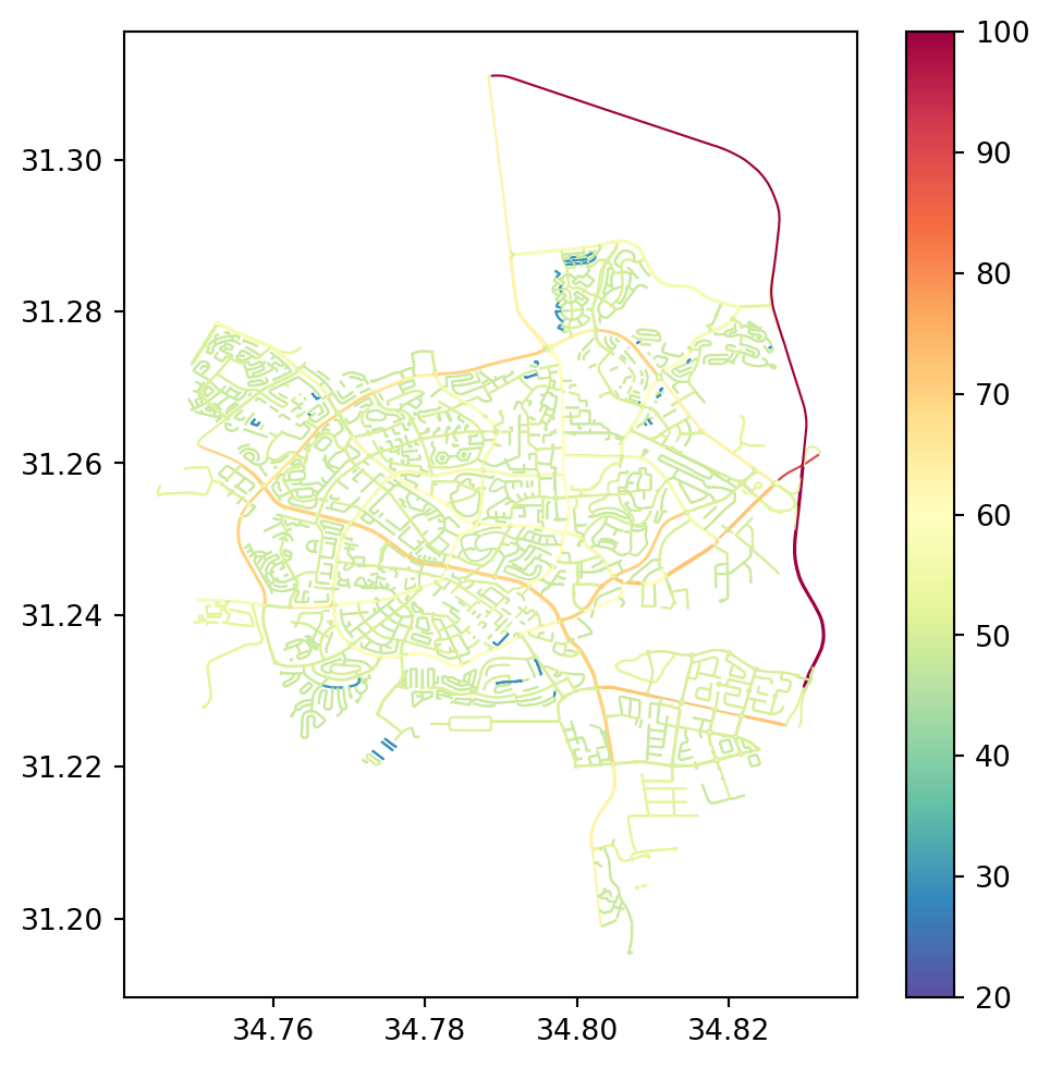

Figure 11.2: Imputed edge speeds in the Beer-Sheva road network

MultiDiGraph to DiGraph

As you may note from the G printout, or explicitly using .is_multigraph (Network type), osmnx creates a network of type MultiDiGraph (see Network types in networkx), to accomodate parallel edges:

G.is_multigraph()

True

In a multi-graph, each edge has a third component—to distinguish between multiple edges that have the same source and destination nodes (i.e., (u,v,key)):

list(G.edges)[0]

(127675195, 1775804621, 0)

However, for simplicity, it is preferable to transform the network to a DiGraph. Before we do that, let’s record the number of edges (including “duplicated” ones) in G:

edges_before = G.number_of_edges()
edges_before

10424

The ox.convert.to_digraph function is used to convert from MultiDiGraph to DiGraph. When there are multiple edges between the given pair of nodes, the function retains just the one edge which minimizes the weight. In this case, we choose to retain the edges with the minimal travel time:

G = ox.convert.to_digraph(G, weight='travel_time')
G

<networkx.classes.digraph.DiGraph at 0x74cacf2fa4b0>

Here is the number of edges in the resulting DiGraph:

edges_after = G.number_of_edges()
edges_after

10344

As shown below, the vast majority of edges were not “duplicated”, therefore the number of edges was not much reduced by the transition from MultiDiGraph to DiGraph:

edges_after / edges_before

0.9923254029163469

And, naturally, the edges are now identified only by the IDs of origin and destination nodes (i.e., (u,v)):

list(G.edges)[0]

(127675195, 1775804621)

Standardizing the network

At this point we can pass our network to the net2.prepare function, for validation purposes, and to standardize towards the structure we are used to. For example, the property name 'travel_time' which osmnx imputes is replaced with simply 'time'.

Here is an example of a specific edge before applying net2.prepare:

G.edges[list(G.edges)[0]]

{'osmid': 605647724,
 'highway': 'primary',
 'name': 'שדרות בנ"צ כרמל',
 'oneway': True,
 'reversed': False,
 'length': np.float64(33.31813479688256),
 'speed_kph': 63.125,
 'travel_time': 1.90012333099053}

Here we apply net2.prepare:

G = net2.prepare(G)
G

<networkx.classes.digraph.DiGraph at 0x74ca8db53e30>

And here is the same edge after applying net2.prepare:

G.edges[list(G.edges)[0]]

{'osmid': 605647724,
 'highway': 'primary',
 'name': 'שדרות בנ"צ כרמל',
 'oneway': True,
 'reversed': False,
 'length': 33.31813479688256,
 'speed_kph': 63.125,
 'time': 1.90012333099053}

Node 'x' and 'y' to 'geometry'

osmnx uses 'x' and 'y' attributes to represent node locations. We are going to convert the information to 'geometry'.

for i in G.nodes:
    G.nodes[i]['geometry'] = shapely.Point(G.nodes[i]['x'], G.nodes[i]['y'])

Deleting unnecessary attributes

An OSM-based network careated using osmnx contains numerous attributes, which are irrelevant for our purposes (i.e., routing). For example, here are the attributes of a specific node and edge from G, respectively:

G.nodes[list(G.nodes)[12]]

{'y': 31.239111,
 'x': 34.7914697,
 'street_count': 4,
 'geometry': <POINT (34.791 31.239)>}

G.edges[list(G.edges)[12]]

{'osmid': 308341908,
 'highway': 'tertiary',
 'maxspeed': '50',
 'name': 'קרן קיימת לישראל',
 'oneway': True,
 'reversed': False,
 'length': 49.04716296207483,
 'geometry': <LINESTRING (34.793 31.237, 34.792 31.237, 34.792 31.238, 34.792 31.238)>,
 'speed_kph': 50.0,
 'time': 3.5313957332693877}

However, not all nodes are guaranteed to contain the same attributes. To systematically collect all possible attributes in all network nodes, we can go over the attributes in a for loop, as follows. Here we see that there are 4 possible node attributes in G:

result = []
for i in G.nodes:
    for a in G.nodes[i].keys():
        if a not in result:
            result.append(a)
result

['y', 'x', 'highway', 'street_count', 'geometry']

Note

A shorter, though more difficult to read, method to do the same is through set comprehension:

{k for i in G.nodes for k in G.nodes[i].keys()}

The same can be done for the edges, in which case we can see that there are many possible attributes:

result = []
for u,v in G.edges:
    for a in G.edges[u,v].keys():
        if a not in result:
            result.append(a)
result

['osmid',
 'highway',
 'name',
 'oneway',
 'reversed',
 'length',
 'speed_kph',
 'time',
 'maxspeed',
 'ref',
 'lanes',
 'geometry',
 'junction',
 'bridge',
 'tunnel']

For simplicity, we are going to keep just the 'geometry' attributes for the nodes. In the following code section, we go over the nodes, then going over the attributes of each node, each time checking whether the current node belongs to the keep list (of node attributes to keep). It the attribite is not in keep—then it is deleted:

keep = ['geometry']
for i in G.nodes:
    for attr in list(G.nodes[i].keys()):
        if attr not in keep: 
            del G.nodes[i][attr]

Similarly, we filter the edge attributes to keep just five important ones:

keep = ['geometry', 'name', 'length', 'speed_kph', 'time']
for u,v in G.edges:
    for attr in list(G.edges[u,v].keys()):
        if attr not in keep: 
            del G.edges[u,v][attr]

Revisiting the specific node and edge shown above demonstrates that indeed they now contain just the selected subset of attributes:

G.nodes[list(G.nodes)[12]]

{'geometry': <POINT (34.791 31.239)>}

G.edges[list(G.edges)[12]]

{'name': 'קרן קיימת לישראל',
 'length': 49.04716296207483,
 'geometry': <LINESTRING (34.793 31.237, 34.792 31.237, 34.792 31.238, 34.792 31.238)>,
 'speed_kph': 50.0,
 'time': 3.5313957332693877}

Dealing with list attributes

As part of network simplification (What is osmnx), some of the network edges may incorporate the properties of several separate road sections. For example, two streets having different names may be combined into one. In such case, the respective property becomes a list. The following code section identifies, and prints, a 'name' attribute of type list of a specific edge:

for u,v in G.edges:
    if 'name' in G.edges[u,v] and isinstance(G.edges[u,v]['name'], list):
        x = G.edges[u,v]['name']
        print(x)
        break

['סמילנסקי משה', 'שלשת בני עין חרוד']

Having list attributes in a network can make it incompatible with certain operations, such as writing it to an '.xml' file (Writing the Beer-Sheva network). To transform a list of names into a str, we may concatenate the names, along with a separating character such as ';':

';'.join(x)

'סמילנסקי משה;שלשת בני עין חרוד'

The following code standardizes all of the 'name' attribute values in the network G according to the following scenarios:

• If the 'name' is missing→assign ' '
• If the 'name' is a list→combine the values into str

for u,v in G.edges:
    if 'name' not in G.edges[u,v]:
        G.edges[u,v]['name'] = ''
    if 'name' in G.edges[u,v] and isinstance(G.edges[u,v]['name'], list):
        G.edges[u,v]['name'] = ';'.join(G.edges[u,v]['name'])

Filling edge geometries

osmnx does not assign the 'geometry' attribute to all edges, but only to those edges where the geometry is more complex than a straight line segment. For that reason, we can see that the 'geometry' is missing in many of the edges:

edges_before = net2.edges_to_gdf(G).geometry
edges_before

0                                      None
1                                      None
2                                      None
                        ...                
10341                                  None
10342    LINESTRING (34.75125 31.23927, ...
10343                                  None
Name: geometry, Length: 10344, dtype: geometry

More specifically, here is how we can calculate the proportion of non-missing geometries:

edges_before.notna().mean()

np.float64(0.6731438515081206)

For consistency, we prefer all edges (as well as all nodes) to have the same complete set of attributes. For example, when converting the network to a line layer, edges without a 'geometry' attribute are going to be missing from the line layer, impeding analysis of the data.

Assuming that the missing 'geometry' attributes should be straight line segments between the respective nodes defining the edge, here is how the 'geometry' attributes can be filled:

for u,v in G.edges:
    e = G.edges[u, v]
    if 'geometry' not in e:
        geom = shapely.LineString([G.nodes[u]['geometry'], G.nodes[v]['geometry']])
        G[u][v]['geometry'] = geom

Looking again at the derived GeoSeries of edge geometries, we can see that it is now complete:

edges_after = net2.edges_to_gdf(G).geometry
edges_after

0        LINESTRING (34.82615 31.25743, ...
1        LINESTRING (34.82615 31.25743, ...
2        LINESTRING (34.79846 31.25076, ...
                        ...                
10341    LINESTRING (34.75125 31.23927, ...
10342    LINESTRING (34.75125 31.23927, ...
10343    LINESTRING (34.7983 31.2342, 34...
Name: geometry, Length: 10344, dtype: geometry

Figure 11.3 shows the line layer of edge geometries before and after filling the missing 'geometry' attributes:

base = edges_after.difference(edges_before.union_all()).plot(color='red', linewidth=0.5);
edges_before.plot(color='blue', linewidth=0.5, ax=base);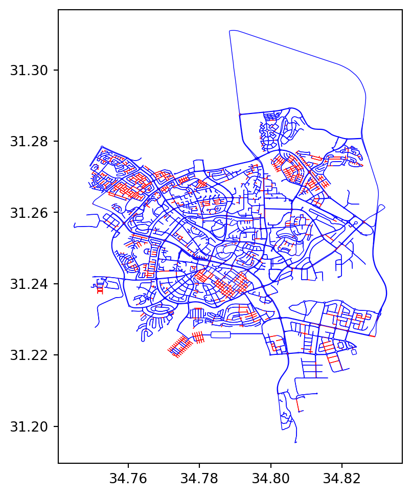

Figure 11.3: The line layer of edge geometries, original (in blue) and the newly calculated parts as a result of filling the missing 'geometry' attributes (in red)

Projecting geometries

For any distance-related workflow, we prefer spatial data to be in a projected CRS. Therefore, we are going to project the road network from WGS84 (EPSG:4326) to UTM (EPSG:32636). Specifically, we need to recalculate the nodes and edges 'geometry' attributes. To do that, we create a “transformer” object (Reprojection (shapely)):

transformer = pyproj.Transformer.from_crs(4326, 32636, always_xy=True)

Suppose that we take just the 1^st edge geometry object x:

x = G.edges[list(G.edges)[0]]['geometry']
print(x)

LINESTRING (34.8261528 31.2574282, 34.8258779 31.2576141)

Here is how we can apply shapely.transform to calculate the corresponding projected geometry:

x = shapely.transform(x, transformer.transform, interleaved=False)
print(x)

LINESTRING (673879.2197105067 3459570.1303395974, 673852.6997891894 3459590.305351978)

Using for loops, we can do the same for all nodes and edges in G:

for i in G.nodes:
    G.nodes[i]['geometry'] = shapely.transform(
        G.nodes[i]['geometry'], 
        transformer.transform, 
        interleaved=False
    )
for u,v in G.edges:
    G.edges[u, v]['geometry'] = shapely.transform(
        G.edges[u, v]['geometry'], 
        transformer.transform, 
        interleaved=False
    )

Let’s demonstrate that the geometry of the first edge was indeed changed:

x = G.edges[list(G.edges)[0]]['geometry']
print(x)

LINESTRING (673879.2197105067 3459570.1303395974, 673852.6997891894 3459590.305351978)

Writing the Beer-Sheva network

To use the Beer-Sheva network in other examples in the book, we export it to an '.xml' file as follows:

H = G.copy()
for i in H.nodes:
    H.nodes[i]['geometry'] = str(H.nodes[i]['geometry'])
for u,v in H.edges:
    H.edges[u, v]['geometry'] = str(H.edges[u, v]['geometry'])
nx.write_graphml(H, 'output/beer-sheva.xml')

To examine the Beer-Sheva road network geometries, we can also export its edges to a '.gpkg' file:

edges = net2.edges_to_gdf(G, crs=32636)
edges.to_file('output/beer-sheva_edges.gpkg')

Routing (OSM)

Now that the network is ready, we can try applying routing calculations to it. For example, suppose that we want to calculate the optimal driving route from the Ramot Sportiv community center, to the Ikea store, in Beer-Sheva. Let’s first define the origin and destination coordinates. We use the (lon,lat) coordinates, which can be obtained through geocoding (Geocoding (osmnx)) or interactively from web maps (such as Google Maps) or GIS software:

orig = shapely.Point(34.799796, 31.281758)  # Ramot Sportiv
dest = shapely.Point(34.822357, 31.225021)  # Ikea
orig, dest

(<POINT (34.8 31.282)>, <POINT (34.822 31.225)>)

Since our networks’ coordinates are in UTM (see Projecting geometries), we need to transform the queried locations accordingly:

orig = shapely.transform(orig, transformer.transform, interleaved=False)
dest = shapely.transform(dest, transformer.transform, interleaved=False)
orig, dest

(<POINT (671325.25 3462225.99)>, <POINT (673577.024 3455971.644)>)

Now we can find the shortest route from orig to dest, as follows:

route = net2.route2(G, orig, dest, 'time')

The total distance (in \(m\)) and travel time (in \(sec\)) can be calculated using nx.path_weight (Sum of route weights):

nx.path_weight(route['network'], route['route'], weight='length')

8854.78665536379

nx.path_weight(route['network'], route['route'], weight='time')

480.7979084409927

To display the route on a map, let’s extract the GeoDataFrame of the route:

route_gdf = net2.route_to_gdf(route['network'], route['route'])
route_gdf

	from	to	geometry
0	-1	7666966450	LINESTRING (671339.356 3462215....
1	7666966450	7666962338	LINESTRING (671319.394 3462189....
2	7666962338	7666991994	LINESTRING (671406.53 3462105.1...
...	...	...	...
58	6586125365	6586082151	LINESTRING (673453.803 3455826....
59	6586082151	6586082152	LINESTRING (673461.624 3455855....
60	6586082152	-2	LINESTRING (673459.942 3455859....

61 rows × 3 columns

Figure 11.4 shows the result:

base = net2.edges_to_gdf(G).plot(linewidth=0.2, color='grey')
gpd.GeoSeries(shapely.Point(orig)).plot(ax=base, color='blue');
gpd.GeoSeries(shapely.Point(dest)).plot(ax=base, color='blue');
route_gdf.plot(ax=base, color='red');

Figure 11.4: Fastest route from Ramot Sportiv to Ikea

For comparison, let’s also find the shortest route between the same two locations. Note that, this time, we minimize 'length' rather than 'time':

route = net2.route2(G, orig, dest, 'length')

Comparing the total distance (in \(m\)) and travel time (in \(sec\)), we can see that the distance is now smaller:

nx.path_weight(route['network'], route['route'], weight='length')

8789.312775350467

but the travel time is longer:

nx.path_weight(route['network'], route['route'], weight='time')

536.8193589519553

Figure 11.5 shows the shortest path we just calculated (compare with Figure 11.4):

route_gdf = net2.route_to_gdf(route['network'], route['route'])
base = net2.edges_to_gdf(G).plot(linewidth=0.2, color='grey')
gpd.GeoSeries(shapely.Point(orig)).plot(ax=base, color='blue');
gpd.GeoSeries(shapely.Point(dest)).plot(ax=base, color='blue');
route_gdf.plot(ax=base, color='red');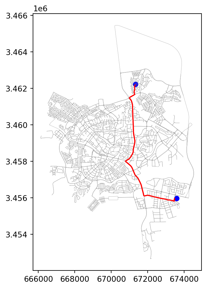

Figure 11.5: Shortest route from Ramot Sportiv to Ikea

Customized regular grid

In Exercise 10-02, we experiment with calculating an accessibility map (Figure 19.23) using the realistic network that we’ve prepared in this chapter. Using the net2.create_grid function (Creating regular grids), here is how we can create a grid of \(500 \times 500\) \(m^2\) cells:

edges = net2.edges_to_gdf(G, crs=32636)
bounds = edges.total_bounds
grid = net2.create_grid(bounds, 500, 32636)
grid

	geometry
0	POLYGON ((666133 3465660, 66663...
1	POLYGON ((666133 3465160, 66663...
2	POLYGON ((666133 3464660, 66663...
...	...
455	POLYGON ((674133 3454160, 67463...
456	POLYGON ((674133 3453660, 67463...
457	POLYGON ((674133 3453160, 67463...

442 rows × 1 columns

Figure 11.6 shows a map of the grid:

base = edges.plot(color='grey', linewidth=0.5, zorder=0)
grid.plot(ax=base, color='none', edgecolor='red', linewidth=0.5, zorder=1);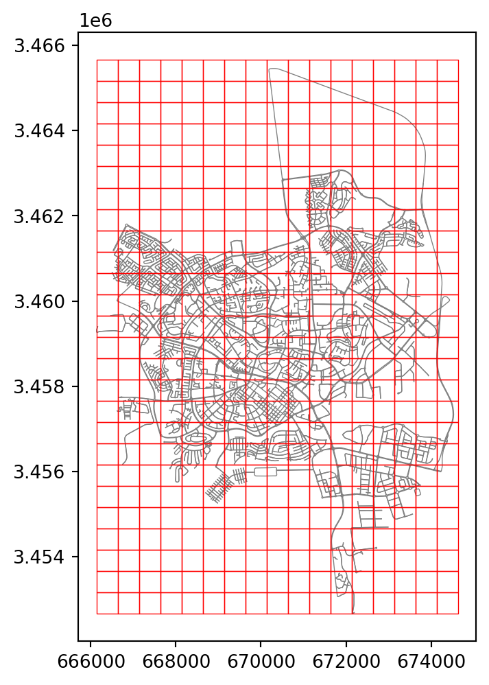

Figure 11.6: A \(500 \times 500\) \(m^2\) grid covering Beer-Sheva

As you can see in Figure 11.6, many of the grid cells are far away from the road network, and therefore practically irrelevant for accessibility calculations. Moveover, we may want to remove grid cells with no points of interest for vehicles to stop at, e.g., along highways. A straightforward approach is to keep only those grid cells which intersect with a buildings layer. osmnx can be used to download a building layer, for a given area of interest, using function ox.features_from_bbox as follows:

buildings = ox.features.features_from_bbox(edges.to_crs(4326).total_bounds, {'building': True})
buildings = buildings.to_crs(32636)

Then, we can subset the grid layer according to intersection (Spatial relations (geopandas)) with (the union of) the buildings layer:

grid = grid[grid.intersects(buildings.union_all())]
grid

	geometry
8	POLYGON ((666133 3461660, 66663...
9	POLYGON ((666133 3461160, 66663...
10	POLYGON ((666133 3460660, 66663...
...	...
425	POLYGON ((673633 3455660, 67413...
447	POLYGON ((674133 3458160, 67463...
449	POLYGON ((674133 3457160, 67463...

201 rows × 1 columns

Figure 11.7 shows the resulting subset of the grid layer, and the buildings layer that was used for subsetting:

base = edges.plot(color='grey', linewidth=0.1, zorder=0)
buildings.plot(ax=base, color='blue')
grid.plot(ax=base, color='none', edgecolor='red', linewidth=0.5, zorder=1);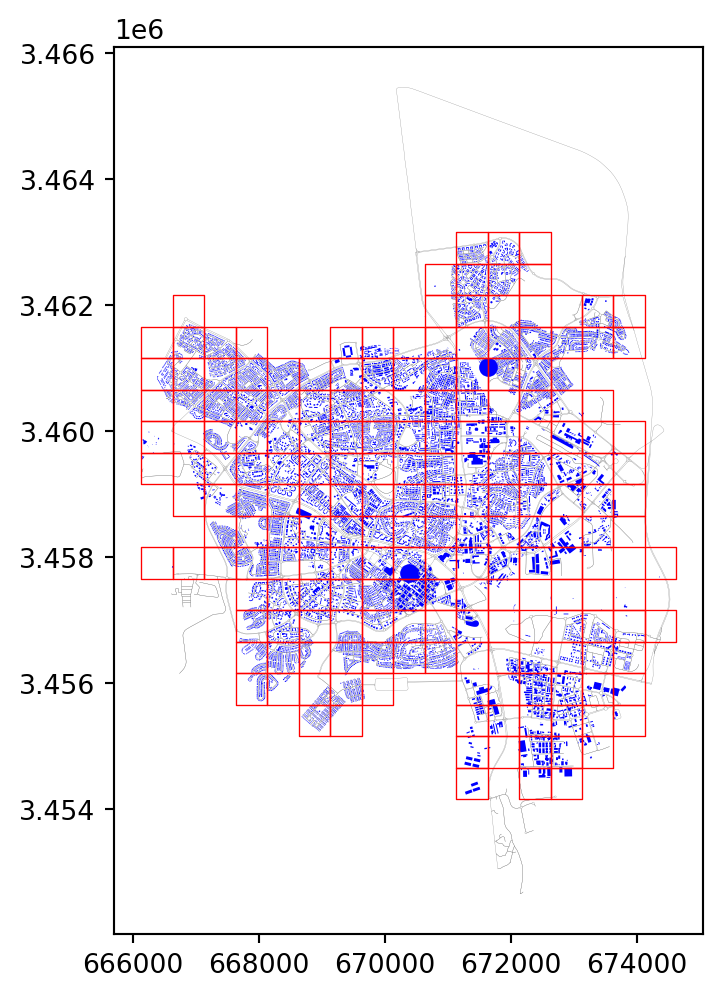

Figure 11.7: A \(500 \times 500\) \(m^2\) grid covering Beer-Sheva, subset according to intersection with the Beer-Sheva buildings layer

Exercises

Exercise 10-01

• Calculate and plot a map of accessibility, in terms of travel time, from one specific location (e.g., Ramot Sportiv) to any other location in Beer-Sheva (Figure 19.22)

Exercise 10-02

• Write a function that accepts:
  • A road network (such as G for Beer-Sheva)
  • The CRS of the network (32636 for the Beer-Sheva network)
  • Origin location name (such as 'Turner Stadium, Beer-Sheva')
  • Destination location name (such as 'Cinema City, Beer-Sheva')
• and returns:
  • The dict with calculated route properties, using net2.route2
• Call the function with specific values and draw a map of Beer-Sheva with the calculated route (Figure 19.23)

Exercise 10-03

• Calculate and plot a route between two points in Beer-Sheva that goes through 'שדרות יצחק רגר' (Figure 19.24)
• Manually modify the attributes in that specific street, by doubling the travel times, simulating a situation of heavy traffic
• Re-calculate and plot the fastest route (Figure 19.25)
• In case the new route is the same as the original one—choose a different pair of points and repeat the exercise

Boeing, Geoff. 2017. “OSMnx: New Methods for Acquiring, Constructing, Analyzing, and Visualizing Complex Street Networks.” Computers, Environment and Urban Systems 65: 126–39. https://doi.org/https://doi.org/10.1016/j.compenvurbsys.2017.05.004.

———. 2025. “Topological Graph Simplification Solutions to the Street Intersection Miscount Problem.” Transactions in GIS 29 (3): e70037.