Last updated: 2026-03-04 01:42:35Accessibility
Introduction
In this chapter, we show how routing calculations can be systematically repeated to develop accessibility metrics, covering the entire surface of the study area. While doing that, we discuss and demonstrate some technical considerations for making repeated routing calculations more accurate and realistic:
We begin with preparing a regular grid covering our sample road network (Regular grids)
We then show how routing calculations can be repeated for all grid cells to obtain accessibility maps, using the basic routing-through-nearest-existing-nodes function (
net2.route1) (Accessibility (1)—Nearest node)We improve the calculation by routing through new nodes inserted into the network where necessary (
net2.route2) (Accessibility (2)—New nodes)To make the map more realistic, we introduce the idea of multi-modal routing, where the route may be composed to different transport modes for different segments (e.g., walking and then driving) (Accessibility (3)—Multi-modal routing)
We then further improve the accessibility map by introducing selection of optimal travel mode (e.g., walking for shorter distances, driving for longer distance) (Accessibility (4)—Optimal mode selection)
Packages
import numpy as np
import pandas as pd
import matplotlib.pyplot as plt
import shapely
import geopandas as gpd
import networkx as nx
import osmnx as ox
import net2
Sample data
Let’s import the sample road network for the examples in this chapter:
G = nx.read_graphml('output/roads2.xml')
G = net2.prepare(G)
G
<networkx.classes.digraph.DiGraph at 0x7e3520bd9c70>Regular grids
For systematically evaluating accessibility, we will create a regular grid covering the extent of the road network. First, we figure out the road network extent:
edges = net2.edges_to_gdf(G)
bounds = edges.buffer(250).total_bounds
bounds
array([-250., -250., 4250., 4250.])Then, we use net2.create_grid (Creating regular grids) to create a regular grid of \(250 \times 250\) \(m^2\) polygons:
grid = net2.create_grid(bounds, 250)
grid| geometry | |
|---|---|
| 0 | POLYGON ((-250 4250, 0 4250, 0 ... |
| 1 | POLYGON ((-250 4000, 0 4000, 0 ... |
| 2 | POLYGON ((-250 3750, 0 3750, 0 ... |
| ... | ... |
| 358 | POLYGON ((4250 250, 4500 250, 4... |
| 359 | POLYGON ((4250 0, 4500 0, 4500 ... |
| 360 | POLYGON ((4250 -250, 4500 -250,... |
361 rows × 1 columns
We also derive the polygon centroids, hereby named ctr:
ctr = grid.centroid
ctr
0 POINT (-125 4125)
1 POINT (-125 3875)
2 POINT (-125 3625)
...
358 POINT (4375 125)
359 POINT (4375 -125)
360 POINT (4375 -375)
Length: 361, dtype: geometryFinally, we define a specific point of interest within the studied extent. In the following sections we are going to calculate maps of travel time to the point, from each location in the studied extent:
pnt = shapely.Point(2800, 200)The road network, polygons grid, centroids ctr, and point pnt, are shown in figure Figure 10.1:
fig, ax = plt.subplots()
grid.plot(ax=ax, color='none', edgecolor='grey')
ctr.plot(ax=ax, color='grey', markersize=1)
plt.plot(pnt.x, pnt.y, 'ro')
nx.draw(G, pos=net2.pos(G), with_labels=True, ax=ax)
plt.axis('on')
ax.tick_params(left=True, bottom=True, labelleft=True, labelbottom=True);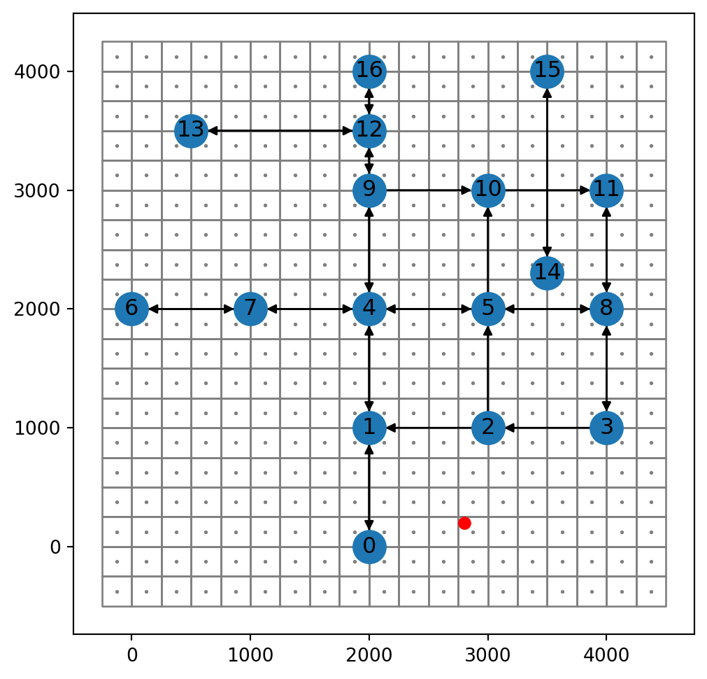
grid, centroids ctr (both in grey), and sample point pnt (in red)
In the following sections we are going to calculate accessibility maps to pnt, using increasingly detailed and realistic methods.
Accessibility (1)—Nearest node
The most basic routing function we wrote, net2.route1 (Basic routing function), calculates the optimal path between two specified existing nodes. For example:
net2.route1(G, 3, 1, 'time'){'route': [3, 8, 5, 4, 1], 'weight': 192.0}When calculating accessiblity, we are referring to specific locations which do not necessarily coincide with a specific node. The simplest solution would be to identify the nearest node, and use that. For example, using our net2.nearest_node function, we can find the nearest node to pnt as follows:
net2.nearest_node(G, pnt)(0, 824.6211251235321)Let’s store the ID in a variable named n:
n = net2.nearest_node(G, pnt)[0]
n0Now, we can go over the ctr points, each time using the net2.route1 function to calculate the travel time from it’s nearest node, to the fixed node n:
result = []
for i in ctr.to_list():
    result.append(net2.route1(G, net2.nearest_node(G, i)[0], n, 'time')['weight'])
The results are collected into a list named result. In the end, the list can be transferred to a new column in the grid layer, named time:
grid['time'] = result
grid| geometry | time | |
|---|---|---|
| 0 | POLYGON ((-250 4250, 0 4250, 0 ... | 248.0 |
| 1 | POLYGON ((-250 4000, 0 4000, 0 ... | 248.0 |
| 2 | POLYGON ((-250 3750, 0 3750, 0 ... | 248.0 |
| ... | ... | ... |
| 358 | POLYGON ((4250 250, 4500 250, 4... | 232.0 |
| 359 | POLYGON ((4250 0, 4500 0, 4500 ... | 232.0 |
| 360 | POLYGON ((4250 -250, 4500 -250,... | 232.0 |
361 rows × 2 columns
Figure 10.2 shows the result, a map of travel times (\(sec\)) to pnt:
fig, ax = plt.subplots(figsize=(8, 5))
grid.plot(column='time', cmap='Spectral_r', legend=True, ax=ax)
nx.draw(G, with_labels=True, pos=net2.pos(G))
plt.plot(pnt.x, pnt.y, 'ro');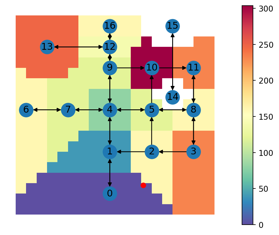
First, as could be expected, you can see that the travel time surface is composed of “blocks” where the value is identical (Figure 10.2). These are groups of cells for which the nearest node on the network is the same—therefore the calculated travel time to pnt is also the same. This issue can be solved by inserting new nodes into the network—which makes the route along the network more accurate. This is what we do next (Accessibility (2)—New nodes).
Second, you can see that there are two distinct areas with “missing” travel time value, apparing white on Figure 10.2. These are the cells for which the nearest node is from a separate network component (14 or 15). Therefore, the route to pnt (node 0) can’t be calculated. We can find out the proportion of cells with missing travel time as follows:
grid['time'].isna().mean()np.float64(0.07202216066481995)Accessibility (2)—New nodes
The last result (Figure 10.2) can be improved by inserting new nodes near the required location, which we learned about in Custom locations. Technically, we use the net2.route2 function (Custom location routing function), which accepts two points rather than two nodes. For example, here is the calculation shown in Figure 9.14:
net2.route2(G, shapely.Point(4100, 3100), shapely.Point(1100, 3700), 'time'){'route': [11, 8, 5, 4, 9, 12, -1],
'weight': 276.8,
'dist_start': 141.4213562373095,
'dist_end': 200.0,
'network': <networkx.classes.digraph.DiGraph at 0x7e352088f140>}Here is how we can apply the calculation over grid:
result = []
for i in ctr.to_list():
    result.append(net2.route2(G, i, pnt, 'time')['weight'])
grid['time'] = result
grid| geometry | time | |
|---|---|---|
| 0 | POLYGON ((-250 4250, 0 4250, 0 ... | 240.0 |
| 1 | POLYGON ((-250 4000, 0 4000, 0 ... | 240.0 |
| 2 | POLYGON ((-250 3750, 0 3750, 0 ... | 240.0 |
| ... | ... | ... |
| 358 | POLYGON ((4250 250, 4500 250, 4... | 224.0 |
| 359 | POLYGON ((4250 0, 4500 0, 4500 ... | 224.0 |
| 360 | POLYGON ((4250 -250, 4500 -250,... | 224.0 |
361 rows × 2 columns
Figure 10.3 shows the resulting travel times:
fig, ax = plt.subplots(figsize=(8, 5))
grid.plot(column='time', cmap='Spectral_r', legend=True, ax=ax)
nx.draw(G, with_labels=True, pos=net2.pos(G))
plt.plot(pnt.x, pnt.y, 'ro');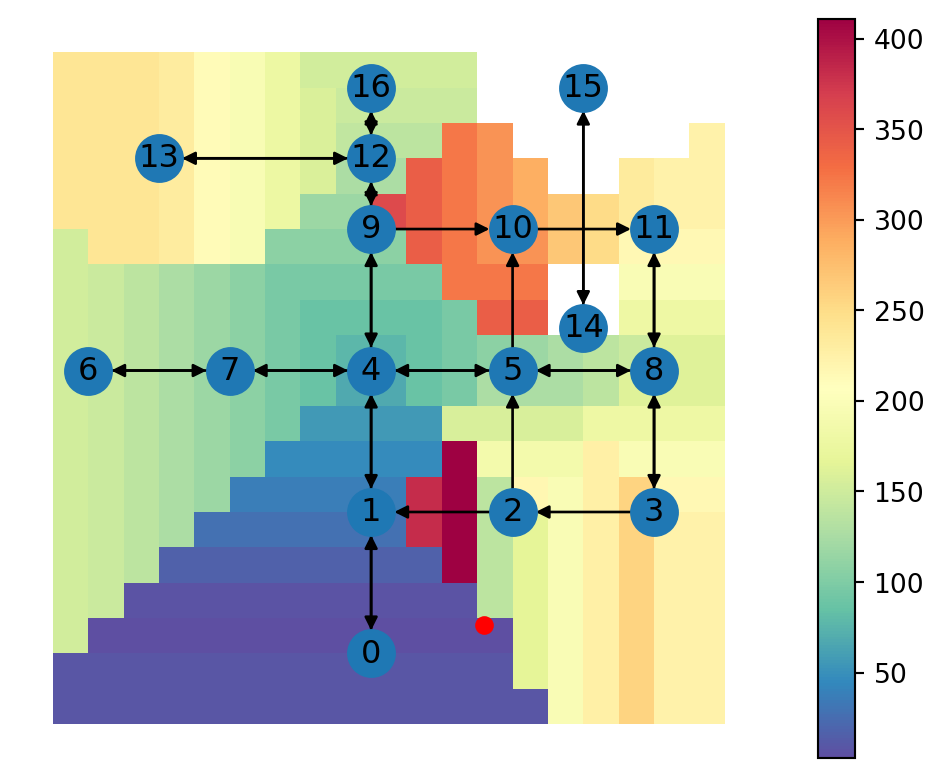
We can now see gradual change of the travel time when moving along the network edges. However, the distance from the starting point to the network itself isn’t being considered. Therefore, for instance, we can see stripes of identical travel time for grid cells sharing the same nearest point along the network. This issue is addressed in the next section (Accessibility (3)—Multi-modal routing).
Accessibility (3)—Multi-modal routing
Multi-modal routing refers to finding an optimal route while combining, and choosing from, several modes of travel, such as driving, walking, and using public transportation. In this section, we will calculate travel time while considering two travel modes:
- Walking
- Driving
Hence, we assume that travel takes place through walking to reach the road network, and then through driving along the road network.
In the following code section, we take into account the additional travel time that it takes to get to and from the road network. We are going to add “walking” times to the travel time calculated using net2.route2.
Assuming a walking speed of 1.4 \(m/s\) (see Tobler’s hiking function), for each calculated route, we sum:
x['weight']—The calculated driving timex['dist_start']/1.4—Walking time from the starting point to the road networkx['dist_end']/1.4—Walking time from the road network to the end point
result = []
for i in ctr.to_list():
    x = net2.route2(G, i, pnt, 'time')
    result.append(x['weight'] + x['dist_start']/1.4 + x['dist_end']/1.4)
grid['time'] = result
grid| geometry | time | |
|---|---|---|
| 0 | POLYGON ((-250 4250, 0 4250, 0 ... | 1442.773912 |
| 1 | POLYGON ((-250 4000, 0 4000, 0 ... | 1332.049276 |
| 2 | POLYGON ((-250 3750, 0 3750, 0 ... | 1266.698171 |
| ... | ... | ... |
| 358 | POLYGON ((4250 250, 4500 250, 4... | 1475.408313 |
| 359 | POLYGON ((4250 0, 4500 0, 4500 ... | 1642.467230 |
| 360 | POLYGON ((4250 -250, 4500 -250,... | 1813.442344 |
361 rows × 2 columns
Figure 10.4 shows the resulting travel times:
fig, ax = plt.subplots(figsize=(8, 5))
grid.plot(column='time', cmap='Spectral_r', legend=True, ax=ax)
nx.draw(G, pos=net2.pos(G), with_labels=True)
plt.plot(pnt.x, pnt.y, 'ro');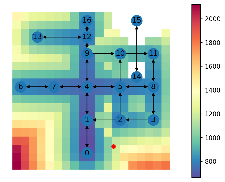
In the Figure 10.4 we can see a more realistic depiction of travel times in the areas far away from the road network. There is one noteable issue, however. In the area directly adjacent the queried point, travel times are unrealistically long, due to the fact that the function only considers travel along the road network, even though a “walking only” route would be faster. This issue brings the idea of multi-modal routing, which we introduce in the next section.
Accessibility (4)—Optimal mode selection
In multi-modal routing, it often makes sense to let the system choose, or at least suggest, an optimal combination of modes, rather than stick to one fixed combination. For example, the last section used the fixed mode combination of walking-driving-walking, which proved to be unrealistic for the areas very close the the queried point (Figure 10.4).
In this section, we are using a new function named net2.route3, which, for the given origin and destination:
- Calculates the walking-driving-walking time, using
net2.route2, as shown in Accessibility (3)—Multi-modal routing - Calculates the walking time, assuming walking in a straight line and walking speed of 1.4 \(m/s\)
- Selects the optimal, i.e., fastest, option, and returns the mode and travel time
In the net2.route3 function definition, first thing being calculated is the straight-line walking time (time_walking). Then, the function attempts to calculate the walking-driving-walking time. Finally, the minimum of the two is determined and returned:
def route3(network, start, end, time_weight, walking_speed=1.4):
    import math
    dist = math.sqrt(((start.x - end.x) ** 2) + ((start.y - end.y) ** 2))
    time_walking = dist / walking_speed
    try:
        result = route2(network, start, end, time_weight)
        time_driving_and_walking = result['dist_start']/walking_speed + result['weight'] + result['dist_end']/walking_speed
    except:
        return {'weight': np.nan, 'mode': np.nan}
    if time_driving_and_walking <= time_walking:
        return {'weight': time_driving_and_walking, 'mode': 'walking+driving'}
    else:
        return {'weight': time_walking, 'mode': 'walking'}
For example, recall the pnt coordinates given a very proximate point, net2.route3 chooses the walking mode, returning the travel time through walking:
net2.route3(G, shapely.Point(3000, 500), pnt, 'time'){'weight': 257.5393768188564, 'mode': 'walking'}When given a point that is far away, net2.route3 chooses the walking+driving+walking mode, returning its travel time:
net2.route3(G, shapely.Point(3000, 3500), pnt, 'time'){'weight': 1224.5714285714284, 'mode': 'walking+driving'}Let’s apply the function over the entire grid:
result = []
for i in ctr.to_list():
    result.append(net2.route3(G, i, pnt, 'time')['weight'])
grid['time'] = result
grid| geometry | time | |
|---|---|---|
| 0 | POLYGON ((-250 4250, 0 4250, 0 ... | 1442.773912 |
| 1 | POLYGON ((-250 4000, 0 4000, 0 ... | 1332.049276 |
| 2 | POLYGON ((-250 3750, 0 3750, 0 ... | 1266.698171 |
| ... | ... | ... |
| 358 | POLYGON ((4250 250, 4500 250, 4... | 1126.274788 |
| 359 | POLYGON ((4250 0, 4500 0, 4500 ... | 1148.701574 |
| 360 | POLYGON ((4250 -250, 4500 -250,... | 1197.627331 |
361 rows × 2 columns
Figure 10.5 shows the resulting travel times:
fig, ax = plt.subplots(figsize=(8, 5))
grid.plot(column='time', cmap='Spectral_r', legend=True, ax=ax)
nx.draw(G, pos=net2.pos(G), with_labels=True)
plt.plot(pnt.x, pnt.y, 'ro');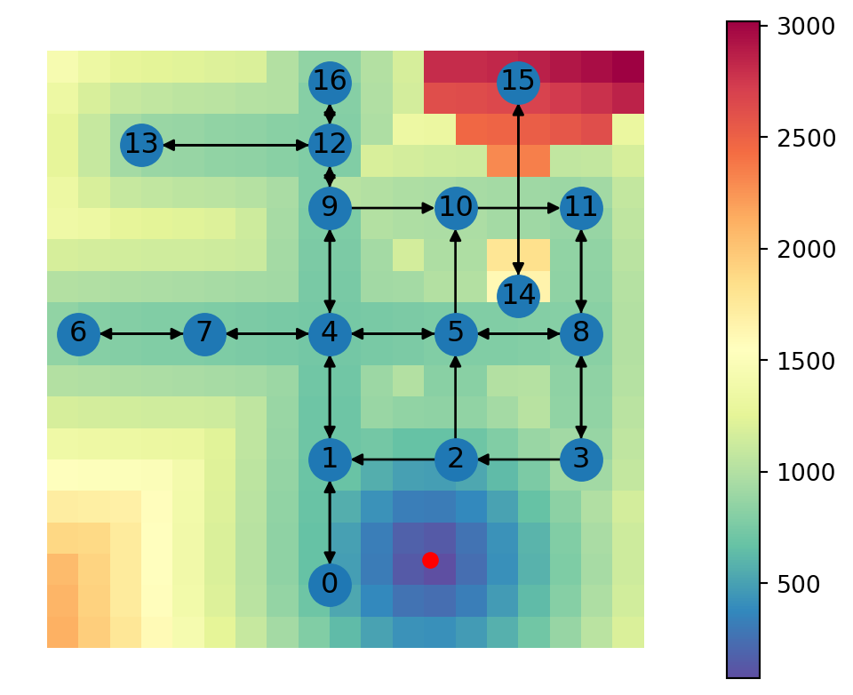
Now we can see that the area around the chosen location is characterized by short travel times through walking, which is more realistic. A map of the selected travel mode, which you are asked to prepare in Exercise 09-02, helps understand the result.
An artefact of the new method, however, is that the area around the disconnected network component (nodes 14 and 15) is now considered “accessible”, but is assigned with very long travel times through walking. Since walking mode is always considered “possible”, that’s what the function chooses in those cases where driving through the network is impossible. Accordingly, we can see that now there are no missing values in the calculated 'time' attribute:
grid['time'].isna().mean()np.float64(0.0)Assuming that the disconnected component is a data preparation issue, the solution is to “connect” it to the network and re-calculate the travel time map. You are asked to do this in Exercise 09-01.
However, if the disconnected component is indeed realistic, the the right routing solution would be to walk (or drive) to the nearest connected component, and go on from there. Or, in general, we can say that sometimes the best option would be to start from a non-nearest node, so that the destination is still reachable through driving, or to acheive a faster travel time. Solving this would require evaluating multiple multi-modal routes, which is beyond the scope of this book.
Note
Here are some more ideas for an improving the accuracy and realism of accessibility calculations, beyond what was shown in this chapter:
- Public transport can be considered as an alternative to driving, thus evaluating accessibility for the part of the population who don’t drive
- We can set a threshold of minimal driving distance, and incorporate some kind of “penalty” time to get in and out of the car. For example, it’s not realistic to drive 100 \(m\) and then walk 20 more \(m\)—people would choose to walk the entire route
Practice
- What would the accessibility map (Figure 10.5) look like, if walking was faster, at 2 \(m/s\)?
- Write a modified version of the
net2.route3function, and re-calculate the accessibility map, to find out
Exercises
Exercise 09-01
- Join the isolated component (nodes
14and15, and the edge between them) to the roads network (see Exercise 07-01) - Recreate the accessibility map shown in Figure 10.5 using the modified network (Figure 19.19)
Exercise 09-02
- Use the modified network from Exercise 09-01
- Display a map of the mode of the fastest route (“walking+driving” or “walking”) (Figure 19.20)
Exercise 09-03
- Use the modified network from Exercise 09-01
- Recreate the accessibility map shown in Figure 10.5 using the modified network and using a twice more detailed (i.e., higher resolution) grid
- Draw a vector layer of contours (i.e., isochrones) for travel times at fixed 500 \(sec\) intervals (i.e.,
500,1000,1500,2000) (Figure 19.21)