Last updated: 2026-03-04 01:42:14Spatial networks
Introduction
In this chapter, we introduce the concept of spatial networks—networks where nodes represent spatial locations, and edges, when present, represent pathways between those locations:
First, we are going to demonstrate the definition of node
'geometry'attributes, representing node spatial coordinates and thus making the network a “spatial” one (Node 'geometry')Next, we will see how spatial arrangement of the nodes can be taken into account in a network plot, making it a map (Graphics: Spatial layout, Graphics: Additional layers)
We move on to the spatial representation of edges, demonstrating the simplest one, namely defining straight line segment geometries (Calculating edge geometries)
We cover the transformation of nodes (Nodes to point layer) and edges (Edges to line layer) to spatial layers of points and lines, respectively
We show an example of exporting (Spatial network to '.xml') and importing (Spatial network from '.xml') a spatial network
We learn how to subset a spatial network by location (Spatial subsetting)
We write functions to find the spatially nearest node (Nearest node) and nearest edge (Nearest edge) to a given point, which we are going to use layer on in routing calculations
Finally, we demonstrate how edge geometries are not necessarily straight line segments, but can be line geometries of any shape (Modifying network geometry)
Packages
import matplotlib.pyplot as plt
import pandas as pd
import shapely
import geopandas as gpd
import networkx as nx
import net2
Sample data 1
Let’s load the continents network from the previous chapter (see Network to '.xml'):
G = nx.read_graphml('output/continents1.xml')
G
<networkx.classes.graph.Graph at 0x7f7cd915a4b0>Node 'geometry'
In a spatial network, the nodes are associated with spatial geometries representing their location. Technically, we are going to represent node locations using an attribute named 'geometry'. The value of that 'geometry' attribute is going to be a shapely geometry (Vector geometries with shapely), typically of type Point.
For example, assuming that nodes in network G represent a point location, we can set the 'geometry' attributes of a given node as follows:
G.nodes['Africa']['geometry'] = shapely.Point(26.8, 1.3)We can see the newly added attribute in the node data:
dict(G.nodes){'Asia': {},
'Africa': {'geometry': <POINT (26.8 1.3)>},
'North America': {},
'South America': {},
'Antarctica': {},
'Europe': {},
'Australia': {}}In the same way, let’s add a 'geometry' attribite to all other nodes:
G.nodes['Asia']         ['geometry'] = shapely.Point(73.1, 39.5)
G.nodes['Australia']    ['geometry'] = shapely.Point(133.1, -24.9)
G.nodes['North America']['geometry'] = shapely.Point(-99.9, 39.6 )
G.nodes['South America']['geometry'] = shapely.Point(-55.4, -20.7)
G.nodes['Europe']       ['geometry'] = shapely.Point(34.3, 53.6 )
G.nodes['Antarctica']   ['geometry'] = shapely.Point(69.0, -76.1)
Graphics: Spatial layout
The nx.draw function accepts a pos argument, a dict of the following form:
{node1: [x, y], node2: [x, y],...}Where node1 and node2 are the nodes, and x and y are the coordinates where they should be drawn.
In a spatial network, the nodes are associated with spatial coordinates, which can be used for plotting. We only need to collect the coordinates into a dict of format shown above. Recall that our input is a dict where each node has a 'geometry' attribute containing a shapely geometry:
dict(G.nodes){'Asia': {'geometry': <POINT (73.1 39.5)>},
'Africa': {'geometry': <POINT (26.8 1.3)>},
'North America': {'geometry': <POINT (-99.9 39.6)>},
'South America': {'geometry': <POINT (-55.4 -20.7)>},
'Antarctica': {'geometry': <POINT (69 -76.1)>},
'Europe': {'geometry': <POINT (34.3 53.6)>},
'Australia': {'geometry': <POINT (133.1 -24.9)>}}Using dict comprehension (dict comprehension), we construct a dict where the keys are node IDs, and the values are lists of the form [x,y] containing node coordinates:
pos = {i: [G.nodes[i]['geometry'].x, G.nodes[i]['geometry'].y] for i in G.nodes}
pos
{'Asia': [73.1, 39.5],
'Africa': [26.8, 1.3],
'North America': [-99.9, 39.6],
'South America': [-55.4, -20.7],
'Antarctica': [69.0, -76.1],
'Europe': [34.3, 53.6],
'Australia': [133.1, -24.9]}Now, the dict named pos can be passed to nx.draw, resulting in a plot with a spatial layout (Figure 6.1):
nx.draw(G, with_labels=True, pos=pos)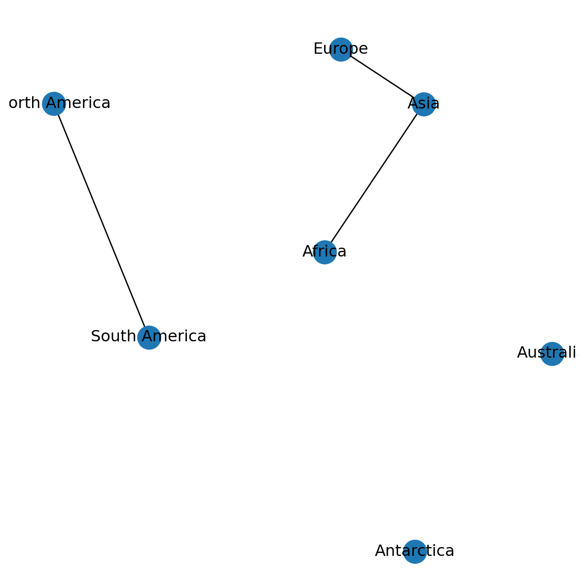
Since we are going to re-use this technique very often, it is worthwhile to define a function, hereby named net2.pos:
def pos(G):
    return {i: [G.nodes[i]['geometry'].x, G.nodes[i]['geometry'].y] for i in G.nodes}
Here is the same plot as shown above, now using the net2.pos function (Figure 6.2):
nx.draw(G, with_labels=True, pos=net2.pos(G))
Graphics: Displaying axes
To display axes on a networkx plot, use the following recipe:
- Initialize the plot with
fig,ax=plt.subplots()to store theaxreference - Plot the network
- Use
plt.axis('on')to initialize the axis lines - Use
ax.set_aspect('equal')for a 1:1 aspect ratio of the x and y axes - Use
ax.tick_params(left=True,bottom=True,labelleft=True,labelbottom=True)for tick mark and labels on the left and bottom axes
Figure 6.3 shows the result:
fig, ax = plt.subplots()
nx.draw(G, with_labels=True, pos=net2.pos(G))
plt.axis('on')
ax.set_aspect('equal')
ax.tick_params(left=True, bottom=True, labelleft=True, labelbottom=True);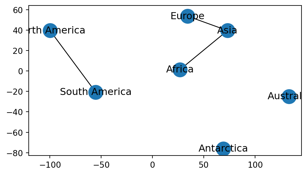
If necessary, you can control the axis limits using the .set_xlim and .set_ylim methods. For example, here is how we can specify a “global” map extent (Figure 6.4):
fig, ax = plt.subplots()
nx.draw(G, with_labels=True, pos=net2.pos(G))
plt.axis('on')
ax.set_aspect('equal')
ax.tick_params(left=True, bottom=True, labelleft=True, labelbottom=True)
ax.set_xlim(xmin=-180, xmax=180)
ax.set_ylim(ymin=-90, ymax=90);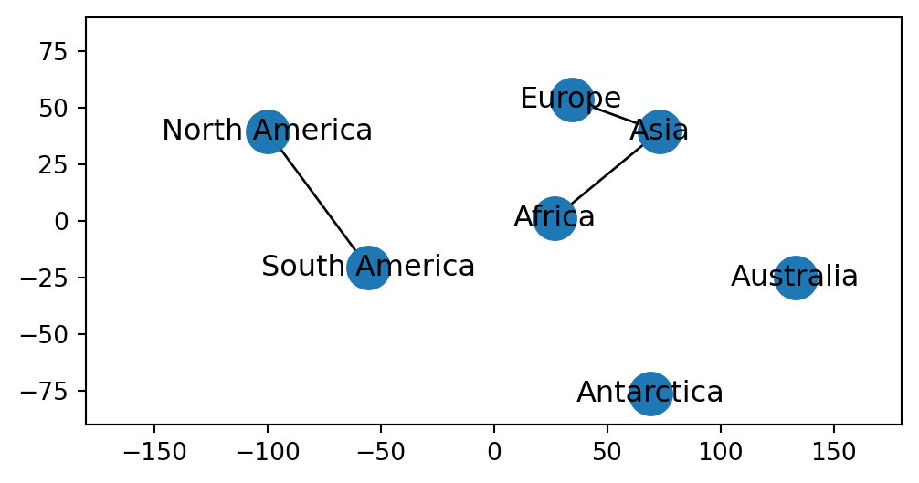
Graphics: Additional layers
Points
We can draw points on top of a networkx plot using plt.plot. We can pass x and y point coordinates as in plt.plot(x,y). The additional 'ro' part in the following example means “red circle”. Here, we are adding a point marker at (0,0) (Figure 6.5):
nx.draw(G, with_labels=True, pos=net2.pos(G))
plt.plot(0, 0, 'ro');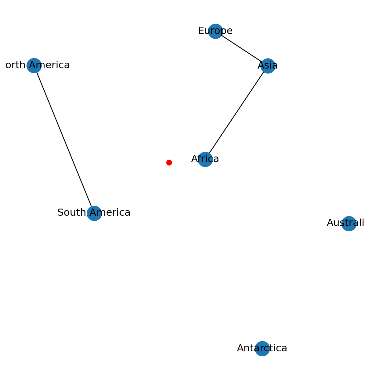
networkx plot with an additional point marker at (0,0)
Polygons
We can draw any other spatial layers in the background of a spatial network plot. For example, let’s import a GeoSeries of country borders:
pol = gpd.read_file('data/ne_110m_admin_0_countries.shp')
pol = pol['geometry']
pol
0 MULTIPOLYGON (((180 -16.06713, ...
1 POLYGON ((33.90371 -0.95, 34.07...
2 POLYGON ((-8.66559 27.65643, -8...
...
174 POLYGON ((20.59025 41.85541, 20...
175 POLYGON ((-61.68 10.76, -61.105...
176 POLYGON ((30.83385 3.50917, 29....
Name: geometry, Length: 177, dtype: geometryThe GeoSeries can be added as background for the nx.draw spatial network plot as follows (Figure 6.6):
pol.plot(color='none', edgecolor='lightgrey')
nx.draw(G, with_labels=True, pos=net2.pos(G))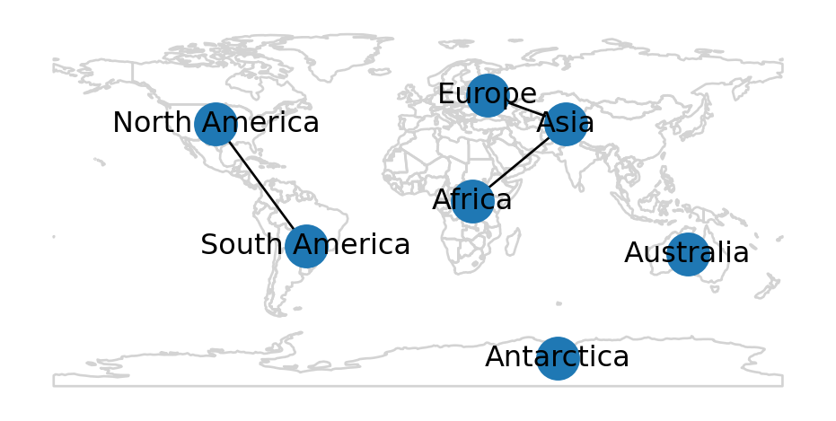
networkx plot with an additional (polygon) layer
Calculating edge geometries
In a spatial network, edges represent connection between spatial locations. In some cases—such as the continents network—the edge shape and placement and shape are arbitrary. In other cases—such as a roads network—however, representing an exact edge geometry is essential. Edge shape, when present, can be represented using a shapely geometry stored in a 'geometry' attribute of every edge.
In cases when edge geometries are absent, it can be helpful to calculate them automatically. In such cases, we assume the edge geometries are straight line segments going from the node u to node v. In terms of code, we can calculate the 'geometry' attributes of all edges by:
- pulling the
'geometry'attributes of nodesuandv, and
- combining the two points to a line geometry with
shapely.LineString(Points to line).
For reference, here are the (empty) attribute dictionary of a specific edge “before” the operation:
G.edges['Asia', 'Africa']{}Here is the code to calculate the geometries:
for u,v in G.edges:
    line = shapely.LineString([G.nodes[u]['geometry'], G.nodes[v]['geometry']])
    G.edges[u, v]['geometry'] = line
And here is the same edge “after” the operation, with the edge geometry:
G.edges['Asia', 'Africa']{'geometry': <LINESTRING (73.1 39.5, 26.8 1.3)>}Network to vector layers
Overview
When working with a spatial network, it is sometimes helpful to extract the nodes and/or the edges as a vector layer. For example, we may want to conduct spatial analysis on the node and edge geometries, to display them on a map, to export them to vector layer files, etc. In this section, we show how to extract vector layer of:
- Node geometries (Nodes to point layer)
- Edge geometries (Edges to line layer)
Nodes to point layer
To extract the nodes to a point vector layer, we go over the nodes in a for loop, collecting the constructed 'Point' geometries along with the node IDs. In the end, the two lists are combined to a GeoDataFrame:
geom = []
node_id = []
for i in G.nodes:
    geom.append(G.nodes[i]['geometry'])
    node_id.append(i)
nodes = gpd.GeoDataFrame({'id': node_id, 'geometry': geom})
nodes| id | geometry | |
|---|---|---|
| 0 | Asia | POINT (73.1 39.5) |
| 1 | Africa | POINT (26.8 1.3) |
| 2 | North America | POINT (-99.9 39.6) |
| ... | ... | ... |
| 4 | Antarctica | POINT (69 -76.1) |
| 5 | Europe | POINT (34.3 53.6) |
| 6 | Australia | POINT (133.1 -24.9) |
7 rows × 2 columns
The resulting GeoDataFrame named nodes is plotted in Figure 6.7:
nodes.plot();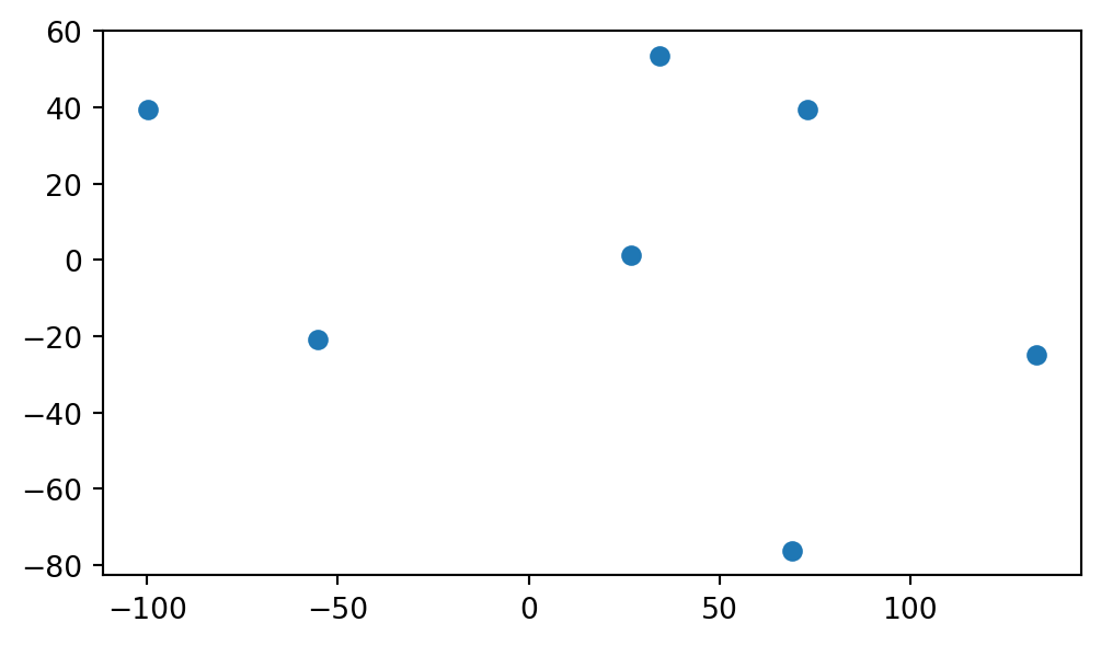
GeoDataFrame extracted from the continents network
The workflow is wrapped into a function named net2.nodes_to_gdf:
def nodes_to_gdf(network, crs=None):
    geom = []
    node_id = []
    for i in network.nodes:
        geom.append(network.nodes[i]['geometry'])
        node_id.append(i)
    nodes = gpd.GeoDataFrame({'id':node_id, 'geometry':geom}, crs=crs)
    return nodes
Note that the function also accepts a crs argument, in case we want the nodes layer to be associated with a CRS. For example:
net2.nodes_to_gdf(G, crs=4326)| id | geometry | |
|---|---|---|
| 0 | Asia | POINT (73.1 39.5) |
| 1 | Africa | POINT (26.8 1.3) |
| 2 | North America | POINT (-99.9 39.6) |
| ... | ... | ... |
| 4 | Antarctica | POINT (69 -76.1) |
| 5 | Europe | POINT (34.3 53.6) |
| 6 | Australia | POINT (133.1 -24.9) |
7 rows × 2 columns
Edges to line layer
To extract the edges to a line vector layer, we can first extract the edges as an “edge list” DataFrame (Network to DataFrame (pandas)):
edges = nx.to_pandas_edgelist(G)
edges| source | target | geometry | |
|---|---|---|---|
| 0 | Asia | Africa | LINESTRING (73.1 39.5, 26.8 1.3) |
| 1 | Asia | Europe | LINESTRING (73.1 39.5, 34.3 53.6) |
| 2 | North America | South America | LINESTRING (-99.9 39.6, -55.4 -... |
Then, assuming that it has a 'geometry' column, the DataFrame can be converted to a GeoDataFrame:
edges = gpd.GeoDataFrame(edges)
edges| source | target | geometry | |
|---|---|---|---|
| 0 | Asia | Africa | LINESTRING (73.1 39.5, 26.8 1.3) |
| 1 | Asia | Europe | LINESTRING (73.1 39.5, 34.3 53.6) |
| 2 | North America | South America | LINESTRING (-99.9 39.6, -55.4 -... |
The GeoDataFrame named edges is plotted in Figure 6.8:
edges.plot();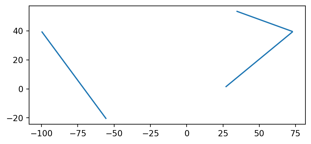
GeoDataFrame extracted from the continents network
The workflow is wrapped into a function named net2.edges_to_gdf:
def edges_to_gdf(network, crs=None):
    edges = nx.to_pandas_edgelist(network)
    edges = gpd.GeoDataFrame(edges, crs=crs)
    return edges
Note that the function also accepts a crs argument, in case we want the edges layer to be associated with a CRS. For example:
net2.edges_to_gdf(G, crs=4326)| source | target | geometry | |
|---|---|---|---|
| 0 | Asia | Africa | LINESTRING (73.1 39.5, 26.8 1.3) |
| 1 | Asia | Europe | LINESTRING (73.1 39.5, 34.3 53.6) |
| 2 | North America | South America | LINESTRING (-99.9 39.6, -55.4 -... |
Note
In this book, we demonstrate creation of a spatial network:
- from scratch (sec-creating-network-object, Sample data 1)
- from
'.xml'file (Sample data 2) - from OpenStreetMap data (OpenStreetMap and osmnx)
Another workflow, which we do not cover in this book, is transforming a line layer (e.g., of roads) into a network. For example, we may want to use a more accurate municipal roads layer rather than OpenStreetMap data. Transforming a line layer into a network is not always straightforward and is associated with its own challenges. For example, the transformation requires that all line segments start and end at nodes representing real intersections, thus distinguished from overpasses, some kind of directionality encoding to tell apart one-way and two-way streets, etc.
Python functions for transforming a line layer into a spatial network include:
osmnx.convert.graph_from_gdfsmomepy.gdf_to_nx(also see Graphs from a set of lines in thenetworkxdocumentation)
Spatial network to '.xml'
When writing a spatial network to '.xml' (Network to '.xml'), we must transform the node and edge geometry attributes to str, as shapely attributes are not supported in nx.write_graphml. For example, here is how we can write G to a file named 'continents2.xml':
for i in G.nodes:
    G.nodes[i]['geometry'] = str(G.nodes[i]['geometry'])
for u,v in G.edges:
    G.edges[u, v]['geometry'] = str(G.edges[u, v]['geometry'])
nx.write_graphml(G, 'output/continents2.xml')
Spatial network from '.xml'
When reading the network back from an '.xml' file, the 'geometry' attributes need to be converted back to shapely, to make it functional (e.g., to calculate edge lengths).
For example, here we import the continents network from the file we’ve just created:
G = nx.read_graphml('output/continents2.xml')
G
<networkx.classes.graph.Graph at 0x7f7cbb071730>The 'geometry' attributes are currently str. For example:
G.nodes['Asia']{'geometry': 'POINT (73.1 39.5)'}G.edges['Asia', 'Africa']{'geometry': 'LINESTRING (73.1 39.5, 26.8 1.3)'}They can be converted to shapely as follows:
for i in G.nodes:
    G.nodes[i]['geometry'] = shapely.from_wkt(G.nodes[i]['geometry'])
for u,v in G.edges:
    G.edges[u, v]['geometry'] = shapely.from_wkt(G.edges[u, v]['geometry'])
The 'geometry' attributes are now shapely:
G.nodes['Asia']{'geometry': <POINT (73.1 39.5)>}G.edges['Asia', 'Africa']{'geometry': <LINESTRING (73.1 39.5, 26.8 1.3)>}Sample data 2
For the other examples in this chapter, we are going to work with a small roads network, stored in the file roads.xml:
G = nx.read_graphml('data/roads.xml')
G
<networkx.classes.graph.Graph at 0x7f7cbb077680>Preparing a spatial network
When reading a spatial network from an '.xml' file exported using nx.write_graphml (Spatial network to '.xml'), there are several checks and transformations we will perform so that the network is ready for further analysis.
First, as shown above (Spatial network from '.xml'), we transform the 'geometry' attributes from str to shapely geometries:
for i in G.nodes:
    G.nodes[i]['geometry'] = shapely.from_wkt(G.nodes[i]['geometry'])
for u,v in G.edges:
    G.edges[u, v]['geometry'] = shapely.from_wkt(G.edges[u, v]['geometry'])
Additionally, note that the node IDs were also imported from the '.xml' file as str:
G.nodesNodeView(('0', '1', '2', '3', '4', '5', '6', '7', '8', '9', '10', '11', '12', '13', '14', '15', '16'))G.edgesEdgeView([('0', '1'), ('1', '2'), ('1', '4'), ('2', '3'), ('2', '5'), ('3', '8'), ('4', '7'), ('4', '5'), ('4', '9'), ('5', '8'), ('5', '10'), ('6', '7'), ('8', '11'), ('9', '10'), ('9', '12'), ('10', '11'), ('12', '13'), ('12', '16'), ('14', '15')])For convenience, we will transform the node IDs to int (assuming they are integers). The nx.relabel_nodes function is used to transform the node IDs, according to the specified “translation”, in this case i→int(i):
mapping = {i: int(i) for i in G.nodes}
mapping
{'0': 0,
'1': 1,
'2': 2,
'3': 3,
'4': 4,
'5': 5,
'6': 6,
'7': 7,
'8': 8,
'9': 9,
'10': 10,
'11': 11,
'12': 12,
'13': 13,
'14': 14,
'15': 15,
'16': 16}G = nx.relabel_nodes(G, mapping)
G<networkx.classes.graph.Graph at 0x7f7cbb075340>Now we can see that the IDs are of type int:
G.nodesNodeView((0, 1, 2, 3, 4, 5, 6, 7, 8, 9, 10, 11, 12, 13, 14, 15, 16))G.edgesEdgeView([(0, 1), (1, 2), (1, 4), (2, 3), (2, 5), (3, 8), (4, 7), (4, 5), (4, 9), (5, 8), (5, 10), (6, 7), (8, 11), (9, 10), (9, 12), (10, 11), (12, 13), (12, 16), (14, 15)])Let’s review the node and edge attributes present in the road network. For the nodes, we have 'geometry' attributes, specifying the node spatial location:
G.nodes[list(G.nodes)[0]]{'geometry': <POINT (2000 0)>}For the edges, we have 'geometry' and 'length':
G.edges[list(G.edges)[0]]{'geometry': <LINESTRING (2000 0, 2000 1000)>, 'length': 1000.0}
Spatial network conventions in this book
- Node IDs are
int - The nodes are associated with:
'geometry'(shapely)
- The edges are associated with:
'geometry'(shapely) (optional)'length'(float) (optional)'time'(float) (optional)
These (and other) preliminary checks and transformations of preparing a spatial network are collectively implemented in the net2.prepare function, which we are going to use from now on:
def prepare(G, ids_to_int=True):
    # IDs to 'int'
    if ids_to_int:
        try:
            mapping = {i: int(i) for i in G.nodes}
            G = nx.relabel_nodes(G, mapping)
        except:
            G = nx.convert_node_labels_to_integers(G, first_label=0)
    # nodes
    for i in G.nodes:
    # 'geometry' to 'shapely'
        if 'geometry' in G.nodes[i]:
            if isinstance(G.nodes[i]['geometry'], str):
                G.nodes[i]['geometry'] = shapely.from_wkt((G.nodes[i]['geometry']))
    # edges
    for u,v in G.edges:
        # 'geometry' to 'shapely'
        if 'geometry' in G[u][v]:
            if isinstance(G[u][v]['geometry'], str):
                G[u][v]['geometry'] = shapely.from_wkt((G[u][v]['geometry']))
        # 'length' to 'float'
        if 'length' in G[u][v]:
            G[u][v]['length'] = float(G[u][v]['length'])
        # rename 'travel_time' to 'time'
        if 'travel_time' in G[u][v]:
            G[u][v]['time'] = G[u][v]['travel_time']
            del G[u][v]['travel_time']
        # 'time' to 'float'
        if 'time' in G[u][v]:
            G[u][v]['time'] = float(G[u][v]['time'])
    return G
Now that the network is ready, we can inspect it visually (Figure 6.9):
fig, ax = plt.subplots()
nx.draw(G, with_labels=True, pos=net2.pos(G))
plt.axis('on')
ax.set_aspect('equal')
ax.tick_params(left=True, bottom=True, labelleft=True, labelbottom=True);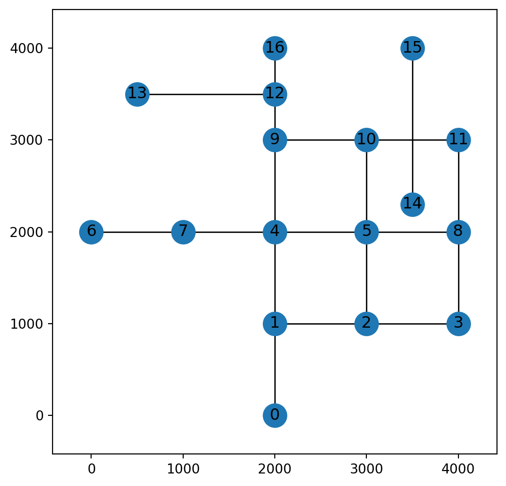
Spatial subsetting
Spatial subsetting of a network is the creation of a sub-network covering a specific area. When creating the spatial subset, we keep just some of the network nodes and/or edges—those that satisfy a spatial condition (Spatial relations (shapely), Spatial relations (geopandas)).
For example, consider the following (rectangular) polygon named pol (Figure 6.10):
pol = shapely.MultiPoint([[1500, 500], [3700, 2500]]).envelope
pol
Figure 6.11 shows the road network G along with the polygon pol. In the example, we are going to subset the nodes, and then the edges, according to intersection with the polygon:
gpd.GeoSeries(pol).plot(color='pink', zorder=0)
nx.draw(G, with_labels=True, pos=net2.pos(G));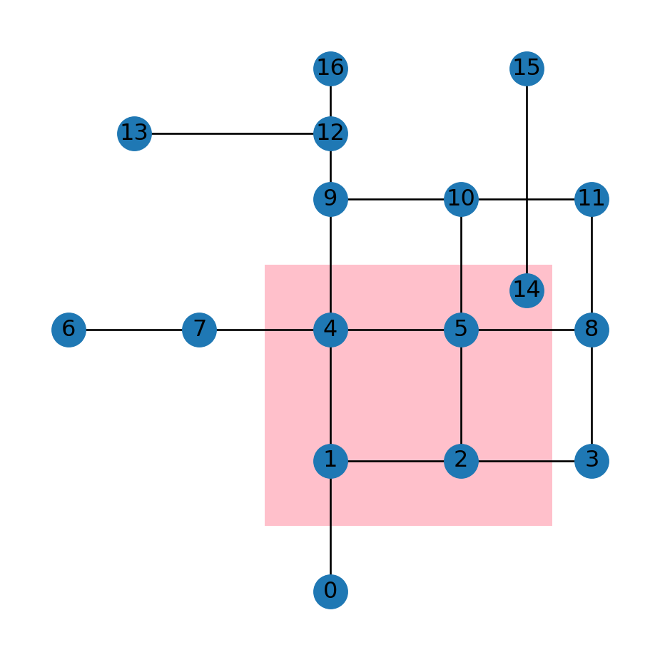
The nx.subgraph_view function can be used to subset a network. nx.subgraph_view accepts filtering functions for parameters filter_node and/or filter_edge. Each of the functions needs to accept a node or an edge, respectively, and return True or False, determing whether to keep it.
For example, here is a function named check_node, which, for each node, constructs the node Point geometry, and then evaluates whether it intersects with pol:
def check_node(node):
    geom = G.nodes[node]['geometry']
    return geom.intersects(pol)
check_node can be passed to nx.subgraph, as a node-filtering function. The result is a sub-network, which we name H:
H = nx.subgraph_view(G, filter_node=check_node)
H
<networkx.classes.graph.Graph at 0x7f7cbb07c1a0>Figure 6.12 shows the network subset H (in red). Naturally, only the edges where both the origin and the destination node are present were retained in H. Recall that an edge specifies the association between existing nodes on a network—therefore an edge cannot be defined without the nodes it refers to.
gpd.GeoSeries(pol).plot(color='pink', zorder=0)
nx.draw(G, with_labels=True, pos=net2.pos(G), node_color='lightgrey', edge_color='lightgrey')
nx.draw(H, with_labels=True, pos=net2.pos(G), node_color='red', edge_color='red', width=3);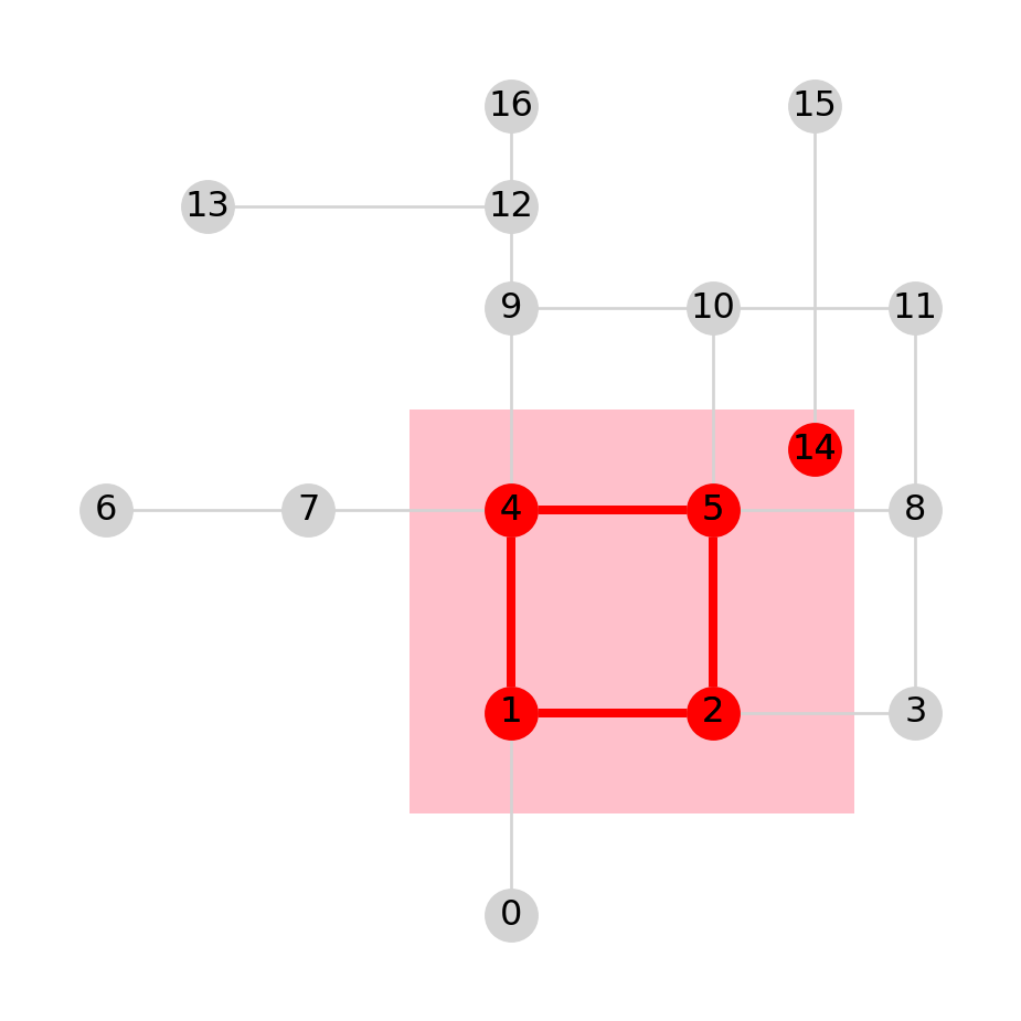
H (in red), creating out of G according to intersection of the nodes with a polygon (in pink)
Practice
- Modify the above code to get a sub-network of
Gwith the nodes that havex<2200, i.e., to the west of the line \(x=2200\).
Now, suppose that we need a more “inclusive” filtering—keeping the edges which intersect, at least partially, with the area of interest (and all of the associated nodes). To subset the required edges, we can use the filter_edge parameter instead of filter_node. The filter_edge function needs to accept the edge IDs u and v, and return a boolean value. The following function check_edge evaluates whether the given edge intersects with the polygon pol:
def check_edge(u, v):
    geom = G.edges[u, v]['geometry']
    return geom.intersects(pol)
Here, we pass the check_edge function to nx.subgraph, as the edge-filtering function. As a result we get a sub-network, which we name I:
I = nx.subgraph_view(G, filter_edge=check_edge)
I
<networkx.classes.graph.Graph at 0x7f7cbb3420c0>Figure 6.13 shows the resulting sub-network, in red. Note how just the edges that intersect with the polygon were retained. However, all of the nodes are retained, since we did not use any node filtering criterion. Unlike the case with edges (Figure 6.12), a node can exist just fine even with no edges referring to it.
gpd.GeoSeries(pol).plot(color='pink', zorder=0)
nx.draw(G, with_labels=True, pos=net2.pos(G), node_color='lightgrey', edge_color='lightgrey')
nx.draw(I, with_labels=True, pos=net2.pos(G), node_color='red', edge_color='red', width=3);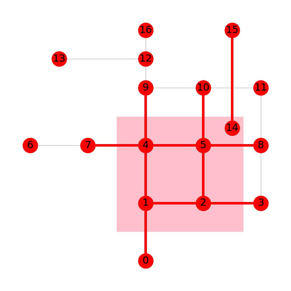
I (in red), creating out of G according to intersection of the edges with a polygon (in pink)
What if we want to keep just those nodes which participate in the selected edges? One way to do that is to remove the isolated nodes. Note that this would remove any isolated nodes within the area of interest too, which we hereby assume are irrelevant too.
To remove the isolated nodes, first we can detect them, using function nx.isolates (Isolated nodes):
i = list(nx.isolates(I))
i
[6, 11, 12, 13, 16]Then, we remove those nodes from network I, using the .remove_nodes_from method. Before doing that, we need to make a copy of the object, using the .copy method. The reason is that nx.subgraph_view returns a read-only view of the subset, which we can’t modify. Once we make a copy using the .copy method, the object is no longer read-only, and can be modified just like an ordinary network object:
I = I.copy()
I.remove_nodes_from(i)
Figure 6.14 shows the modified network I:
gpd.GeoSeries(pol).plot(color='pink', zorder=0)
nx.draw(G, with_labels=True, pos=net2.pos(G), node_color='lightgrey', edge_color='lightgrey')
nx.draw(I, with_labels=True, pos=net2.pos(G), node_color='red', edge_color='red', width=3);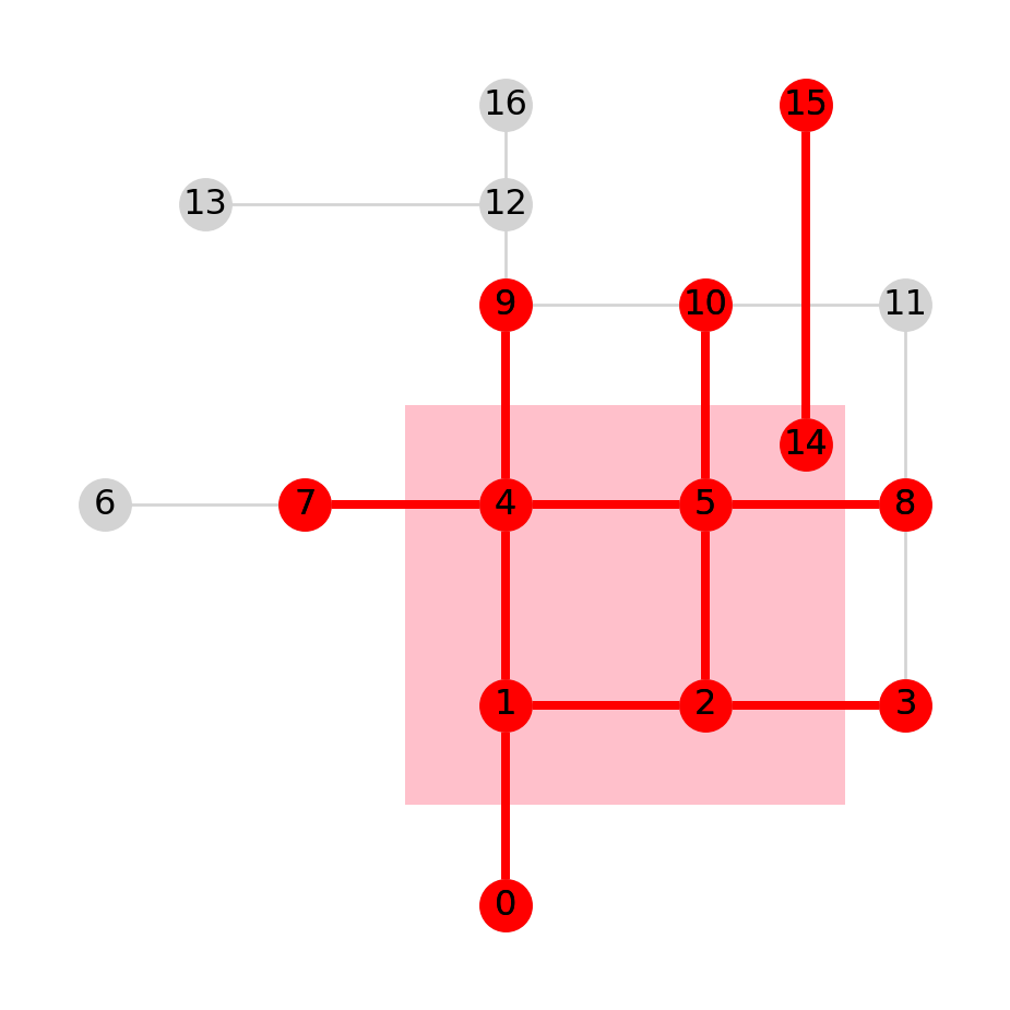
I (in red) from Figure 6.13, with isolated nodes removed
Nearest node or edge
Nearest node
In spatial analysis of networks, and particularly in routing (Routing), we are often required to locate the node which is nearest to a particular location. Let’s demonstrate how this can be done.
Suppose that our location of interest is pnt:
pnt = shapely.Point(1100, 3750)
pnt
Figure 6.15 shows the location of point pnt on top of the network G:
nx.draw(G, with_labels=True, pos=net2.pos(G))
plt.plot(pnt.x, pnt.y, 'go', markersize=10);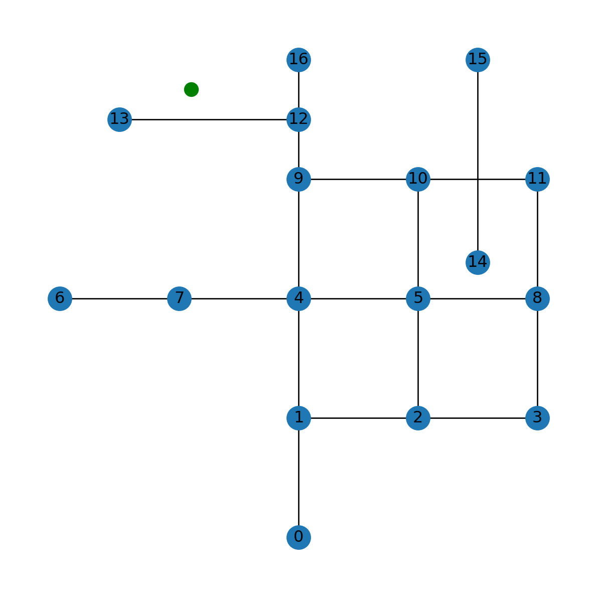
pnt with respect to network G
Now, we need to locate the nearest node to pnt on the road network G. The workflow is as follows:
- Go over all nodes in
G, using aforloop - For each node, calculate the distance to
pnt - The distance is compared to a variable named
min_distance, which holds the up-to-date minimal distance - If distance of the current node is smaller than
min_distance—we updatemin_distanceand record the ID of the node where the new record was found, innearest_node.
When the for loop ends, going through all of the nodes, min_distance and nearest_node hold the distance and ID of the nearest node, respectively.
Before the loop starts, we initialize both min_distance and nearest_node. min_distance is initialized as infinity (why?):
min_distance = float('inf')
min_distanceinfwhereas nearest_node is initially empty:
nearest_node = None
nearest_node
Now, we can run the for loop, as follows:
for i in G.nodes:
    distance = pnt.distance(G.nodes[i]['geometry'])
    if distance < min_distance:
        min_distance = distance
        nearest_node = i
Here are the resulting nearest node ID:
nearest_node13and the distance from it to pnt:
min_distance650.0Figure 6.16 shows the point pnt, in green, and the detected nearest node, in red:
nx.draw(G, with_labels=True, pos=net2.pos(G), node_color='lightgrey', edge_color='lightgrey')
plt.plot(pnt.x, pnt.y, 'go', markersize=10)
plt.plot(G.nodes[nearest_node]['geometry'].x, G.nodes[nearest_node]['geometry'].y, 'ro', markersize=20);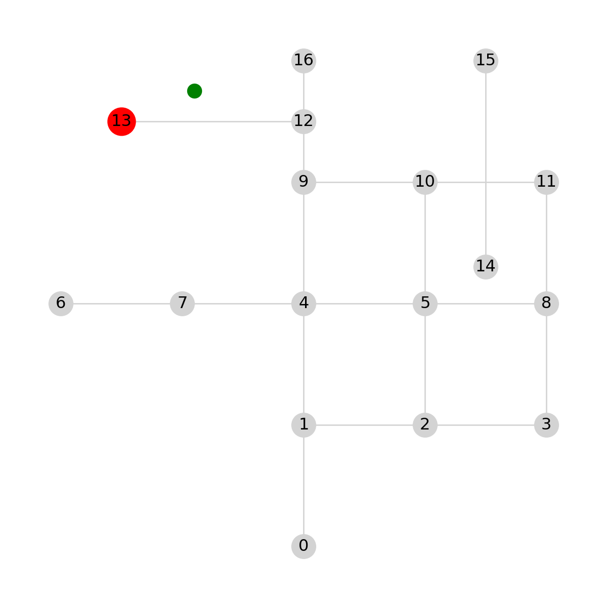
pnt (in green) and the detected nearest node (in red)
The above workflow is wrapped into a function named net2.nearest_node, which we are going to use later on:
def nearest_node(G: nx.Graph, pnt: shapely.geometry.Point) -> tuple:
    min_distance = float('inf')
    nearest_node = None
    for i in G.nodes:
        distance = pnt.distance(G.nodes[i]['geometry'])
        if distance < min_distance:
            min_distance = distance
            nearest_node = i
    return nearest_node, min_distance
Here is a demonstration of the net2.nearest_node function using the same data as above:
net2.nearest_node(G, pnt)(13, 650.0)We can apply the net2.nearest_node function on a regular grid of over the entire spatial extent of the network, to create a map of nearest nodes and distances to them. First, let’s create a regular polygonal grid named grid (Creating regular grids):
edges = net2.edges_to_gdf(G)
bounds = edges.buffer(250).total_bounds
grid = net2.create_grid(bounds, 100)
grid| geometry | |
|---|---|
| 0 | POLYGON ((-250 4250, -150 4250,... |
| 1 | POLYGON ((-250 4150, -150 4150,... |
| 2 | POLYGON ((-250 4050, -150 4050,... |
| ... | ... |
| 2113 | POLYGON ((4250 -50, 4350 -50, 4... |
| 2114 | POLYGON ((4250 -150, 4350 -150,... |
| 2115 | POLYGON ((4250 -250, 4350 -250,... |
2116 rows × 1 columns
and extract the grid centroids ctr:
ctr = grid.centroid
ctr
0 POINT (-200 4200)
1 POINT (-200 4100)
2 POINT (-200 4000)
...
2113 POINT (4300 -100)
2114 POINT (4300 -200)
2115 POINT (4300 -300)
Length: 2116, dtype: geometryNow we can go over the ctr coordinates, each time applying net2.nearest_node for the current centroid i. Inside the for loop, we collect the nearest node identities into nearest_node, and their respective distances to the centroid—into min_distance:
min_distance_node = []
nearest_node = []
for i in ctr.to_list():
    result = net2.nearest_node(G, i)
    nearest_node.append(result[0])
    min_distance_node.append(result[1])
The results can then be attached, as new attributes, to the grid layer:
grid['nearest_node'] = nearest_node
grid['min_distance_node'] = min_distance_node
grid| geometry | nearest_node | min_distance_node | |
|---|---|---|---|
| 0 | POLYGON ((-250 4250, -150 4250,... | 13 | 989.949494 |
| 1 | POLYGON ((-250 4150, -150 4150,... | 13 | 921.954446 |
| 2 | POLYGON ((-250 4050, -150 4050,... | 13 | 860.232527 |
| ... | ... | ... | ... |
| 2113 | POLYGON ((4250 -50, 4350 -50, 4... | 3 | 1140.175425 |
| 2114 | POLYGON ((4250 -150, 4350 -150,... | 3 | 1236.931688 |
| 2115 | POLYGON ((4250 -250, 4350 -250,... | 3 | 1334.166406 |
2116 rows × 3 columns
Figure 6.17 shows a map of the nearest node IDs for each grid cell:
grid.plot(column='nearest_node', cmap='Spectral', legend=True)
nx.draw(G, with_labels=True, pos=net2.pos(G))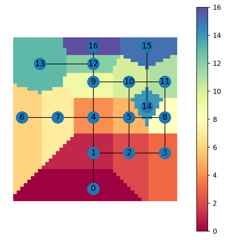
Figure 6.18 shows a map of the distance to the nearest node:
grid.plot(column='min_distance_node', cmap='Spectral', legend=True)
nx.draw(G, with_labels=True, pos=net2.pos(G))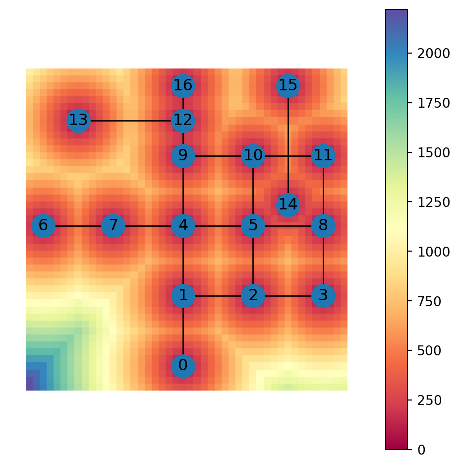
Nearest edge
An analogous useful task is finding the nearest edge, rather than nearest node (Nearest node). The workflow is almost identical, except that instead of constructing the node geometry with shapely.Point, we take use existing edge geometry, i.e., G.edges[i]['geometry'] for each edge i:
min_distance_edge = float('inf')
nearest_edge = None
for i in G.edges:
    distance = pnt.distance(G.edges[i]['geometry'])
    if distance < min_distance_edge:
        min_distance_edge = distance
        nearest_edge = i
As a result, we get the ID of the nearest edge, named nearest_edge:
nearest_edge(12, 13)And the distance to it, min_distance:
min_distance650.0Figure 6.19 shows the point pnt, in green, and the detected nearest edge, in red:
nx.draw(G, with_labels=True, pos=net2.pos(G))
plt.plot(pnt.x, pnt.y, 'go', markersize=10)
nx.draw_networkx_edges(G, pos=net2.pos(G), edgelist=[nearest_edge], edge_color='r', width=3);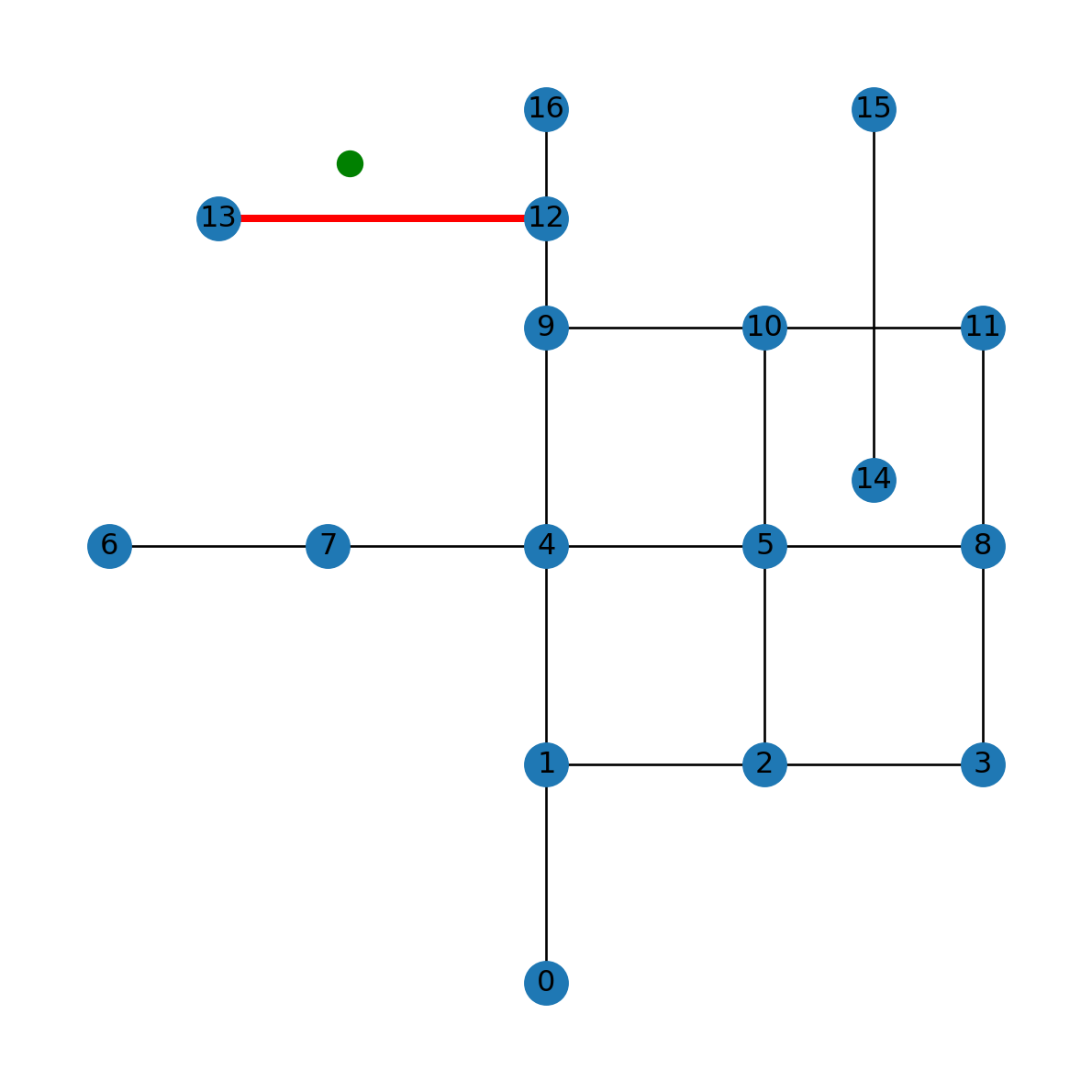
pnt (in green) and the detected nearest edge (in red)
We wrap this workflow into a function named net2.nearest_edge:
def nearest_edge(G: nx.Graph, pnt: shapely.geometry.Point) -> tuple:
    min_distance = float('inf')
    nearest_edge = None
    for i in G.edges:
        geom_edge = G.edges[i]['geometry']
        distance = pnt.distance(geom_edge)
        if distance < min_distance:
            min_distance = distance
            nearest_edge = i
    return nearest_edge, min_distance
Here is a demonstration of the net2.nearest_edge function using the same data as above:
net2.nearest_edge(G, pnt)((12, 13), 250.0)Let’s apply the function on a regular grid over the study area, to demonstrate how it works in various locations:
min_distance_edge = []
nearest_edge = []
for i in ctr.to_list():
    result = net2.nearest_edge(G, i)
    nearest_edge.append(result[0])
    min_distance_edge.append(result[1])
The resulting nearest edge ID and distance can then be attached the the grid layer, as new attributes 'nearest_edge' and 'min_distance_edge', respectively:
grid['nearest_edge'] = nearest_edge
grid['min_distance_edge'] = min_distance_edge
grid| geometry | nearest_node | min_distance_node | nearest_edge | min_distance_edge | |
|---|---|---|---|---|---|
| 0 | POLYGON ((-250 4250, -150 4250,... | 13 | 989.949494 | (12, 13) | 989.949494 |
| 1 | POLYGON ((-250 4150, -150 4150,... | 13 | 921.954446 | (12, 13) | 921.954446 |
| 2 | POLYGON ((-250 4050, -150 4050,... | 13 | 860.232527 | (12, 13) | 860.232527 |
| ... | ... | ... | ... | ... | ... |
| 2113 | POLYGON ((4250 -50, 4350 -50, 4... | 3 | 1140.175425 | (2, 3) | 1140.175425 |
| 2114 | POLYGON ((4250 -150, 4350 -150,... | 3 | 1236.931688 | (2, 3) | 1236.931688 |
| 2115 | POLYGON ((4250 -250, 4350 -250,... | 3 | 1334.166406 | (2, 3) | 1334.166406 |
2116 rows × 5 columns
Figure 6.20 shows a map of the nearest edge IDs for each grid cell (the additional legend_kwds argument shifts the legend outside of the plot area so that it doesn’t obscure it):
grid.plot(column='nearest_edge', cmap='Spectral', legend=True, legend_kwds={'loc':'center left','bbox_to_anchor':(1,0.5)})
nx.draw(G, with_labels=True, pos=net2.pos(G))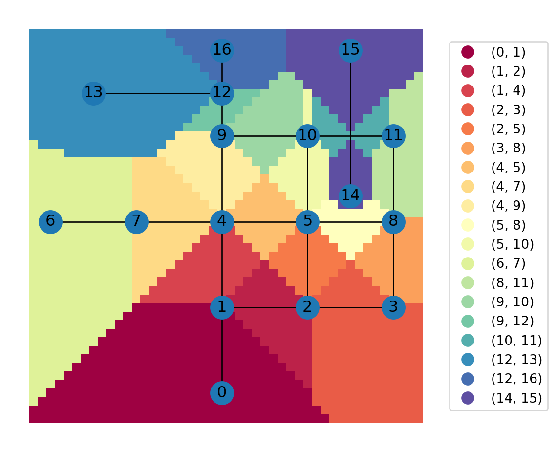
Figure 6.21 shows a map of the distance to the nearest edge:
grid.plot(column='min_distance_edge', cmap='Spectral', legend=True)
nx.draw(G, with_labels=True, pos=net2.pos(G))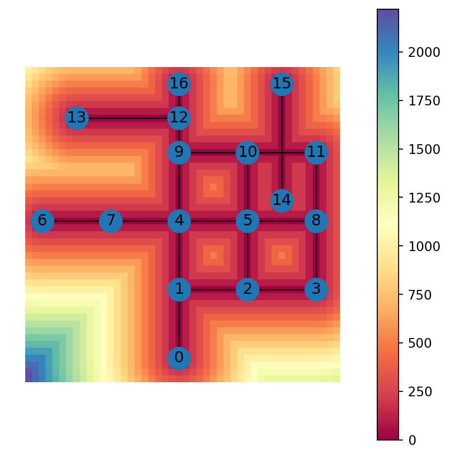
Note
There are existing functions ox.distance.nearest_nodes and ox.distance.nearest_edges, which can also be used to find the nearest network node or edge, respectively. These functions require specifying the CRS, even an arbitrary one, for the network. Otherwise the function assumes lon/lat and gives incorrect distances.
Modifying network geometry
Sometimes the need arises to modify the geometry of the spatial network. For example, it may be necessary to change the geometry of an existing node, e.g., to reflect a change in the shape of the road in the real world.
Note
Another example of modifying network geometry is incorporating a new node on the network, in the middle of an existing edge. This would require:
- “splitting” the exising edge into two new ones,
- removing the original edge
- adding the new node
This procedure is the topic of Custom locations.
In the following example, we demonstrate modifying an existing edge geometry, without otherwise altering the edges and nodes. For example, consider the specific edge 10-11:
G.edges[10,11]{'geometry': <LINESTRING (3000 3000, 4000 3000)>, 'length': 1000.0}The current edge geometry is a straight line:
line1 = G.edges[10,11]['geometry']
line1
Suppose that this specific road segment needs to be replaced with the following, more complex, line geometry:
line2 = shapely.from_wkt('LINESTRING(3000 3000,3200 3200,3800 3200,4000 3000)')
line2
In terms of code, what we need to do is to assign the new geometry into the 'geometry' property of the respective edge:
G.edges[10,11]['geometry'] = line2We can observe the modified edge geometry when transforming the edges to a GeoDataFrame and plotting them (Figure 6.22):
base = net2.edges_to_gdf(G).plot()
net2.nodes_to_gdf(G).plot(ax=base, markersize=200);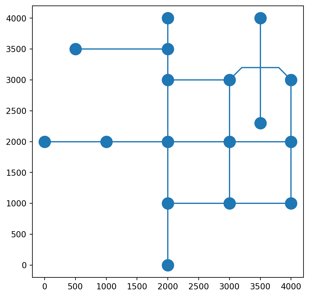
Keep in mind that all of the other edge properties are kept as-is. It is our responsibility to examine which of the other edge properties are out-of-date once the 'geometry' has changed, and updating them. In the case of the roads network, we know that the 'length' attribute should reflect the length of the road segment, but for the computer 'length' is just a generic numeric attribute. Therefore, once the segment geometry has changed, the length is no longer correct:
G.edges[10,11]{'geometry': <LINESTRING (3000 3000, 3200 3200, 3800 3200, 4000 3000)>,
'length': 1000.0}We can update the length of the modified edge as follows:
G.edges[10,11]['length'] = G.edges[10,11]['geometry'].length
G.edges[10,11]
{'geometry': <LINESTRING (3000 3000, 3200 3200, 3800 3200, 4000 3000)>,
'length': 1165.685424949238}Another issue to consider is that when plotting a network using nx.draw, all nodes are drawn as straight-line segments. The nx.draw function is not “aware” of the 'geometry' attribute. Therefore, when plotting the modified network using nx.draw, the edge with the complex 'geometry' attribute is still being drawn as a straight-line segment:
nx.draw(G, with_labels=True, pos=net2.pos(G))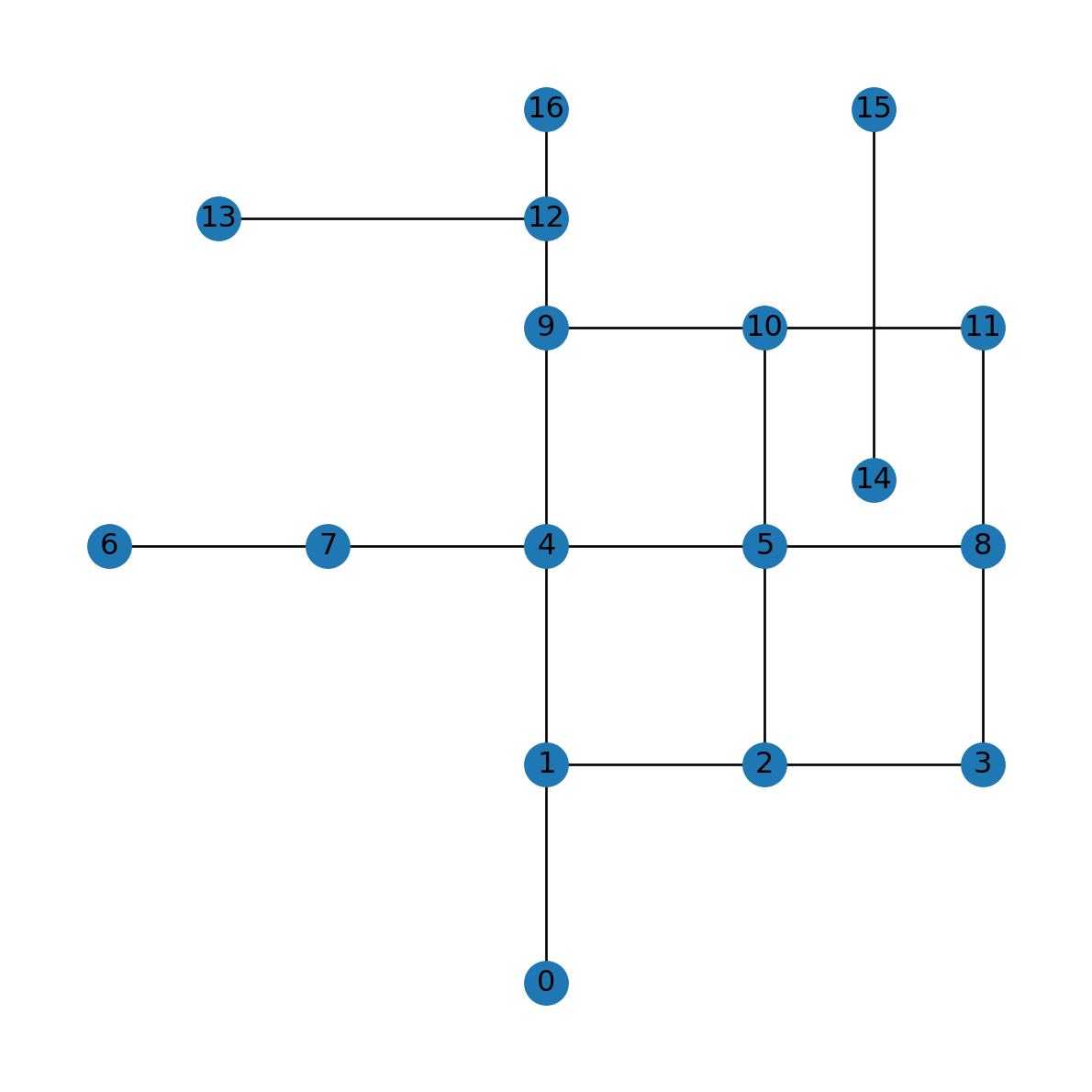
nx.draw where the modification is not reflected
Exercises
Exercise 05-01
- Re-create the railway lines network from Exercise 04-02
- Use geocoding (Geocoding (osmnx)) and reprojection (Reprojection (shapely)) to assign a
'geometry'attributes with'Point'geometries in a suitable projected CRS (e.g.,EPSG:32636) to all stations - Draw a spatial plot of the network (Figure 19.6)
Exercise 05-02
- Calculate and plot, for the road network:
- The betweenness centrality of all nodes (Figure 19.7)
- The degree centrality of all nodes (Figure 19.8)
Exercise 05-03
- Transform the Europe borders network to a spatial one, by adding
'geometry'attributes to all nodes, according to country centroids - Add edge
'geometry'attributes, with straight lines between the respective centroids - Plot the network, together with the country borders (Figure 19.9)