Solutions

Last updated: 2026-03-04 01:47:21

Solution 01-01

[[0.8672246533111945, 0.6438421292004636],
 [0.07574495172138951, 0.13084657283678924],
 [0.4443287285569485, 0.6332320437095613],
 [0.5575327066349794, 0.39278066054598815],
 [0.6824640446594663, 0.4557950762848606],
 [0.14800190799388802, 0.6545227584039292],
 [0.4879925503002518, 0.16194753026651687],
 [0.917920572825771, 0.5891970909478906],
 [0.7766615643664004, 0.4116257688466979],
 [0.7392103667274275, 0.7146024612175764]]

Solution 01-02

[1, 0, 0]

Solution 02-01

array([[  1,   2,   3,   4,   5,   6,   7,   8,   9,  10],
       [  2,   4,   6,   8,  10,  12,  14,  16,  18,  20],
       [  3,   6,   9,  12,  15,  18,  21,  24,  27,  30],
       [  4,   8,  12,  16,  20,  24,  28,  32,  36,  40],
       [  5,  10,  15,  20,  25,  30,  35,  40,  45,  50],
       [  6,  12,  18,  24,  30,  36,  42,  48,  54,  60],
       [  7,  14,  21,  28,  35,  42,  49,  56,  63,  70],
       [  8,  16,  24,  32,  40,  48,  56,  64,  72,  80],
       [  9,  18,  27,  36,  45,  54,  63,  72,  81,  90],
       [ 10,  20,  30,  40,  50,  60,  70,  80,  90, 100]])

Solution 02-02

[34.562429, 34.94056, 29.554168, 31.663251]

Solution 02-03

Table 19.1: Six European countries with the highest number of neighbors

	name	count
12	Germany	9
30	Serbia	8
38	Russia	8
14	Hungary	7
1	Austria	7
36	Ukraine	7

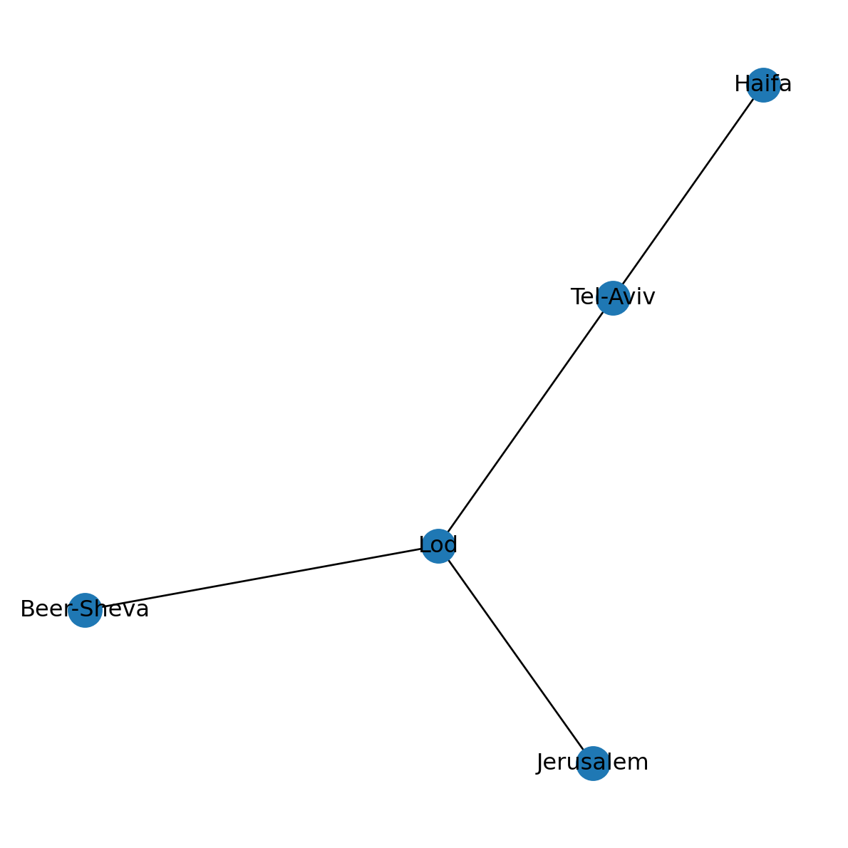
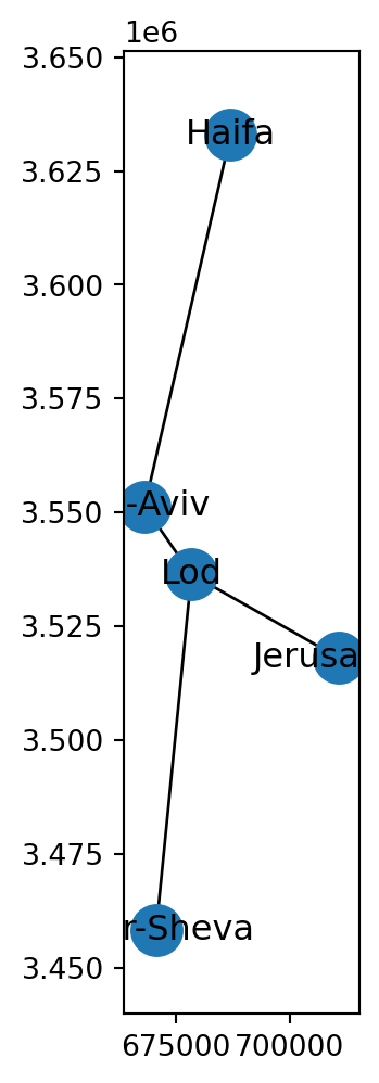
Solution 03-01

Figure 19.1: France borders, and buffers using three different widths: 100, 200, and 300 \(km\)

Solution 03-02

Table 19.2: Distance to ten nearest countries of Spain

	name	dist_km
11	France	0.000000
28	Portugal	0.000000
17	Italy	381029.376539
35	Switzerland	485335.895633
12	Germany	670501.991578
37	United Kingdom	711267.143675
1	Austria	725674.020163
21	Luxembourg	805327.653584
3	Belgium	809999.970891
16	Ireland	885231.173008

Solution 03-03

Figure 19.2: Grand Canyon DEM with the lowest point marked in red

Solution 04-01

Figure 19.3: Students network plot

Solution 04-02

Figure 19.4: Rail network plot

Solution 04-03

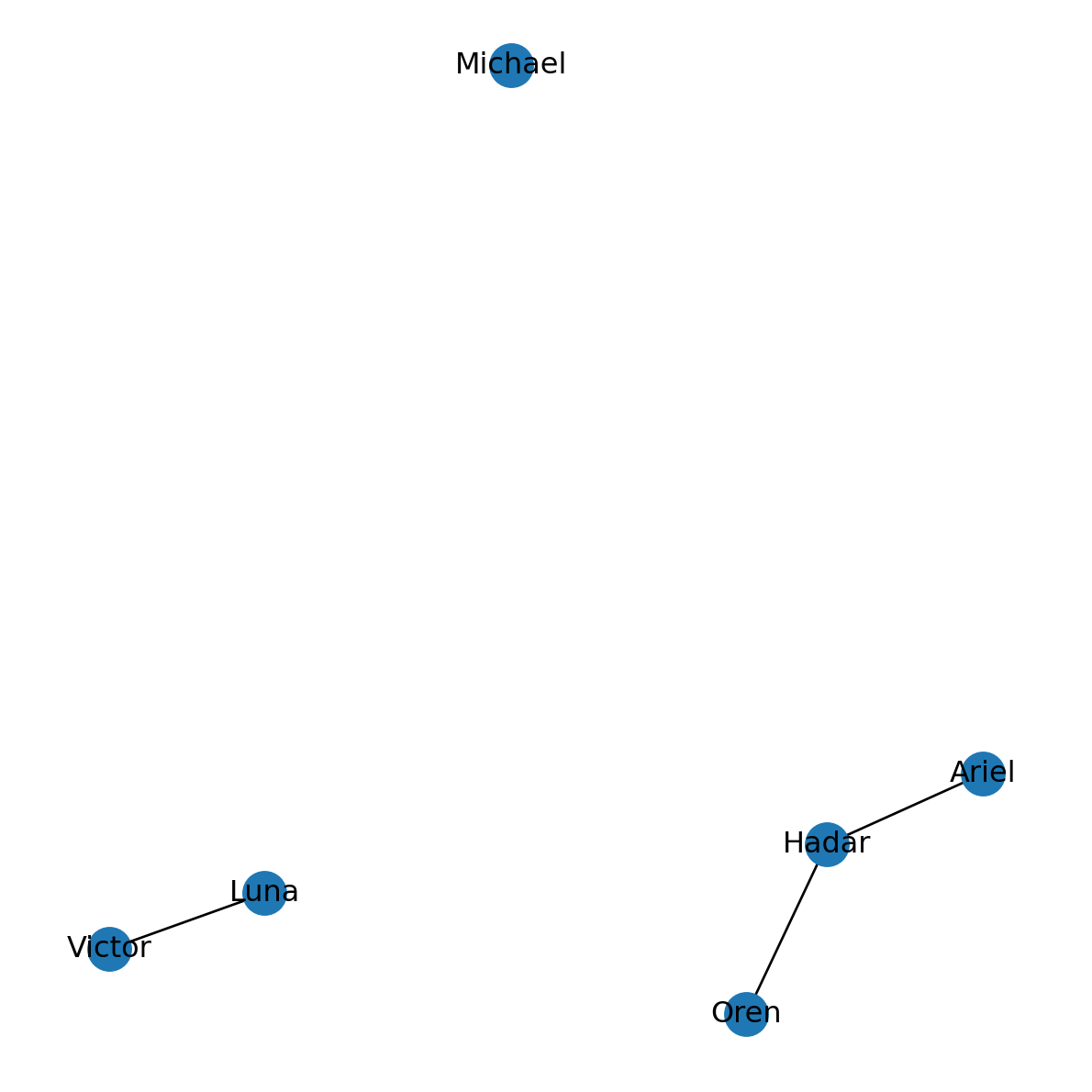
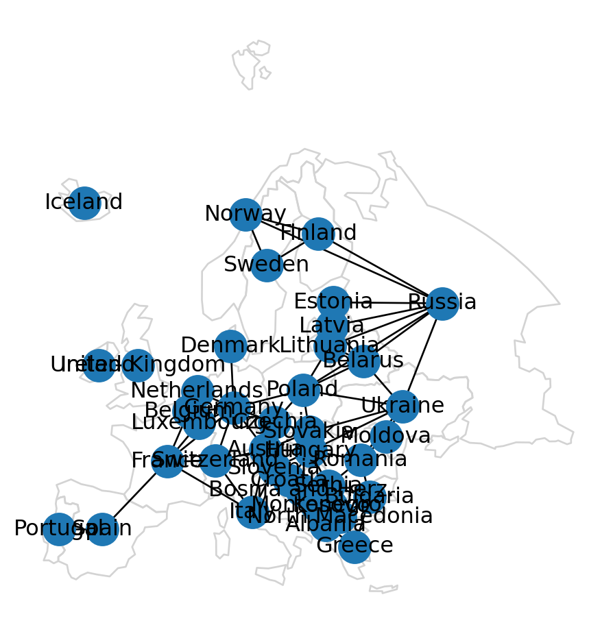
Maximum degree:

('Germany', 9)

Maximum betweenness centrality:

('Germany', 0.24786941365888732)

Number of components (original):

3

Number of components (modified):

1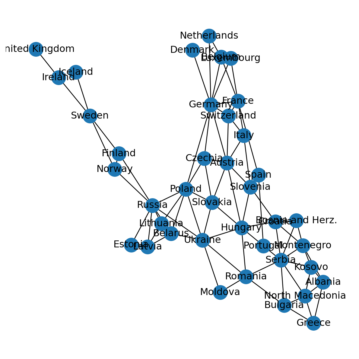

Figure 19.5: Modified European countries network plot

Solution 05-01

Figure 19.6: Rail network plot, with a spatial layout

Solution 05-02

Figure 19.7: Betweenness centrality in the roads network

Figure 19.8: Degree centrality in the roads network

Solution 05-03

Figure 19.9: Spatial layout of the European borders network, with country borders in the background

Solution 06-01

Figure 19.10: Directional network with four nodes and four edges

Solution 06-02

Figure 19.11: Rail network plot, with a spatial layout

Solution 06-03

import matplotlib.pyplot as plt
import pandas as pd
import geopandas as gpd
import networkx as nx
import net2

# Table
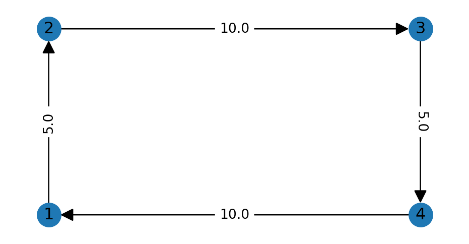
dat = pd.DataFrame({
    'origin': ['France','France','Spain','Spain','Italy','Italy'],
    'destination': ['Spain','Italy','Italy','France','Spain','France'],
    'value': [4628, 15020, 33736, 91923, 278, 5546],
})
dat

	origin	destination	value
0	France	Spain	4628
1	France	Italy	15020
2	Spain	Italy	33736
3	Spain	France	91923
4	Italy	Spain	278
5	Italy	France	5546

# To network
G = nx.from_pandas_edgelist(dat, source='origin', target='destination', edge_attr='value', create_using=nx.DiGraph)
G

<networkx.classes.digraph.DiGraph at 0x74cff332b6b0>

({'France': {'geometry': <POINT (3744078.981 2626928.516)>},
  'Spain': {'geometry': <POINT (3164983.039 2018927.205)>},
  'Italy': {'geometry': <POINT (4507495.567 2177607.133)>}},
 {('France', 'Spain'): {'value': 4628},
  ('France', 'Italy'): {'value': 15020},
  ('Spain', 'Italy'): {'value': 33736},
  ('Spain', 'France'): {'value': 91923},
  ('Italy', 'Spain'): {'value': 278},
  ('Italy', 'France'): {'value': 5546}})

[0.68512, 1.1008, 1.84944, 4.17692, 0.51112, 0.72184]

{('France', 'Spain'): '4,628',
 ('France', 'Italy'): '15,020',
 ('Spain', 'Italy'): '33,736',
 ('Spain', 'France'): '91,923',
 ('Italy', 'Spain'): '278',
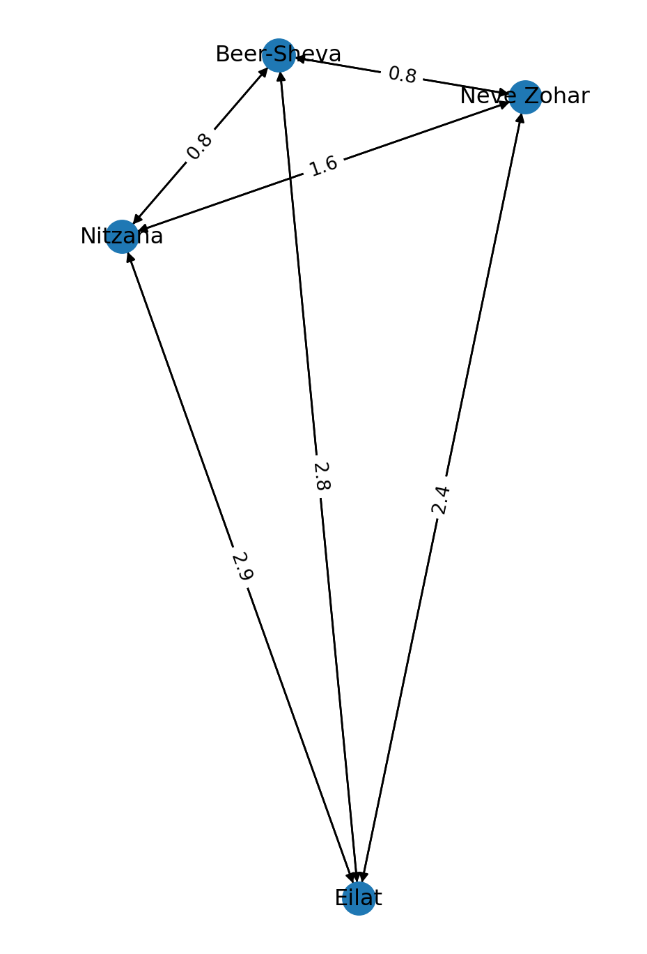
 ('Italy', 'France'): '5,546'}

<Figure size 288x288 with 0 Axes>

<Figure size 288x288 with 0 Axes>

# Plot
pol.plot(color='none', edgecolor='lightgrey')
nx.draw(G, with_labels=True, pos=net2.pos(G), width=weights, connectionstyle='arc3,rad=0.1')
nx.draw_networkx_edge_labels(G, net2.pos(G), labels, connectionstyle='arc3,rad=0.1', font_size=8);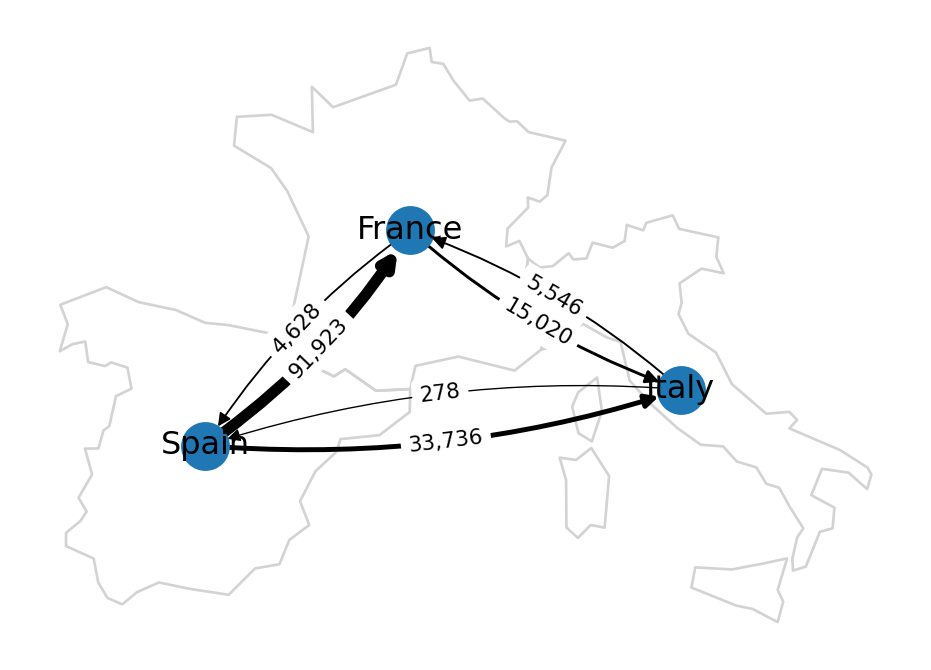

Figure 19.12: Tomato trade volume between three European countries in 2020

Solution 07-01

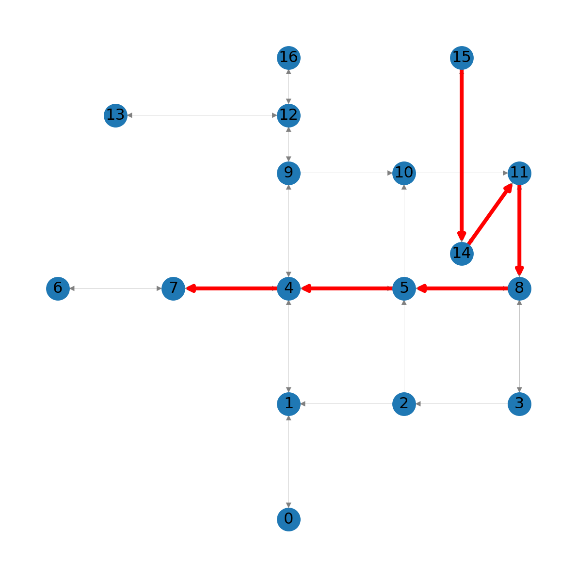
Figure 19.13: fastest route from node 15 to node 7 in the modified road network

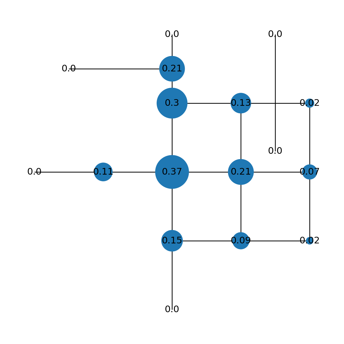
Solution 07-02

Figure 19.14: fastest route from node Haifa to Jerusalem in the railway network

using "nx.path_weight":  83.4706491371249

manual calculation:  83.4706491371249

Solution 07-03

import networkx as nx
import net2

# Network
G = nx.read_graphml('output/roads2.xml')
G = net2.prepare(G)
G

<networkx.classes.digraph.DiGraph at 0x74cff2effef0>

# Travel times
node_labels = {}
sizes = []
for i in G.nodes:
    try:
        route = nx.shortest_path(G, 0, i, weight='time')
        time = nx.path_weight(G, route, weight='time')
    except nx.NetworkXNoPath:
        time = -1
    time = round(time)
    node_labels[i] = time
    sizes.append(time * 3)

# Edge labels
weights = nx.get_edge_attributes(G, 'time')
edge_labels = {k:int(v) for k,v in weights.items()}

# Plot
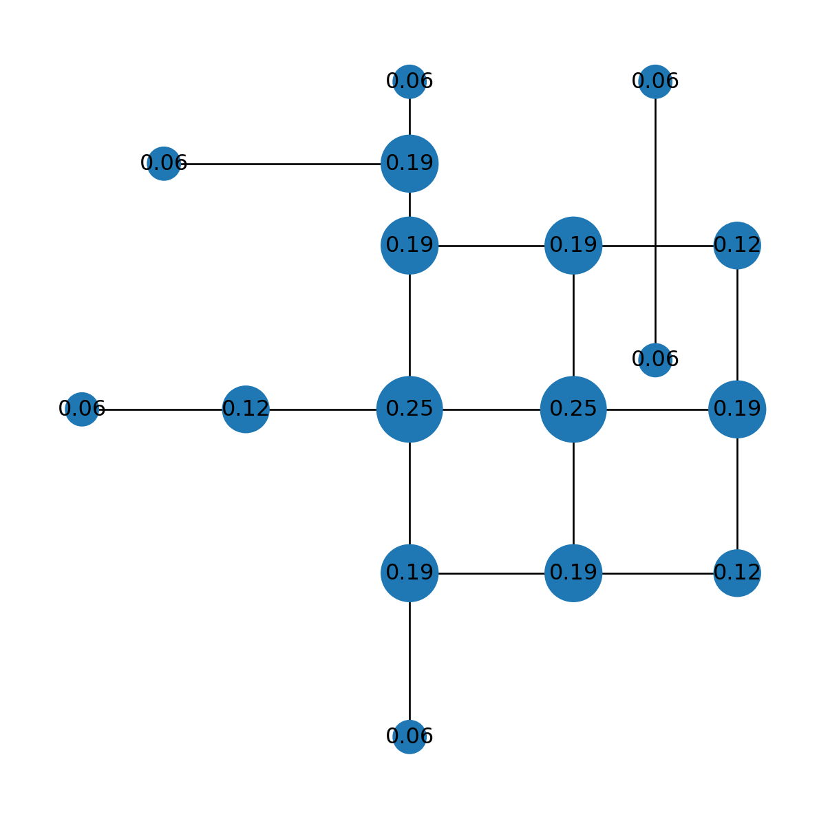
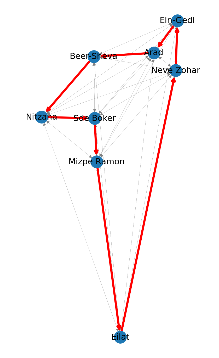
nx.draw(G, pos=net2.pos(G), node_size=sizes)
nx.draw_networkx_labels(G, pos=net2.pos(G), labels=node_labels)
nx.draw_networkx_edge_labels(G, net2.pos(G), edge_labels);

/home/michael/Sync/venv/m/lib/python3.12/site-packages/matplotlib/collections.py:999: RuntimeWarning: invalid value encountered in sqrt
  scale = np.sqrt(self._sizes) * dpi / 72.0 * self._factor
/home/michael/Sync/venv/m/lib/python3.12/site-packages/networkx/drawing/nx_pylab.py:672: RuntimeWarning: invalid value encountered in sqrt
  return self.np.sqrt(marker_size) / 2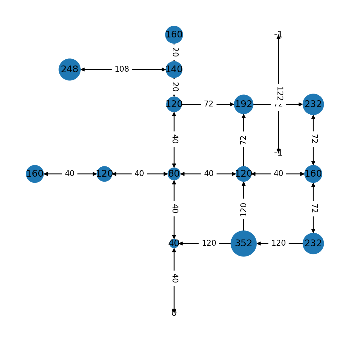

Figure 19.15: Travel times from node 0 to all other nodes. Travel time of -1 marks unreachable nodes

Solution 08-01

Figure 19.16: Shortest route Netanya to Beer-Sheva, by interting new node into the rail network

Solution 08-02

import numpy as np
import shapely
import geopandas as gpd
import networkx as nx
import net2

# Read network
G = nx.read_graphml('output/roads2.xml')
G = net2.prepare(G)
G

<networkx.classes.digraph.DiGraph at 0x74cff2cdff80>

# Generate random points
edges = net2.edges_to_gdf(G)
bounds = edges.buffer(250).total_bounds
xmin, ymin, xmax, ymax = bounds
points = []
while len(points) < 300:
    random_point = shapely.Point([np.random.uniform(xmin, xmax), np.random.uniform(ymin, ymax)])
    points.append(random_point)

# Plot
base = gpd.GeoSeries(points).plot(color='red')
nx.draw(G, pos=net2.pos(G), with_labels=True, edge_color='lightgrey', node_color='lightgrey', ax=base);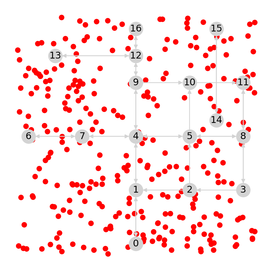

Figure 19.17: Road network and 250 random points

# Calculate and draw segments
lines = []
points2 = []
for i in points:
    result = net2.add_node(G, i)
    pnt2 = result[0].nodes[result[1]]
    points2.append(pnt2['geometry'])
    line = shapely.LineString([i, pnt2['geometry']])
    lines.append(line)
lines = gpd.GeoSeries(lines)
points2 = gpd.GeoSeries(points2)

# Plot
base = gpd.GeoSeries(points).plot(color='red', markersize=10, zorder=1)
lines.plot(ax=base, color='black', linewidth=1, zorder=1)
points2.plot(ax=base, color='blue', markersize=10, zorder=1)
net2.nodes_to_gdf(G).plot(ax=base, color='lightgrey', zorder=-1)
net2.edges_to_gdf(G).plot(ax=base, color='lightgrey', zorder=-1);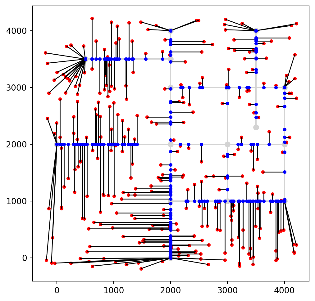

Figure 19.18: New nearest nodes added to the road network (blue) for combining it with random locations (red)

Solution 08-03

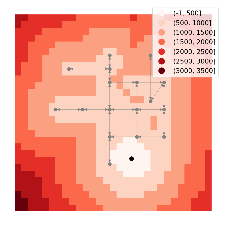
Solution 09-01

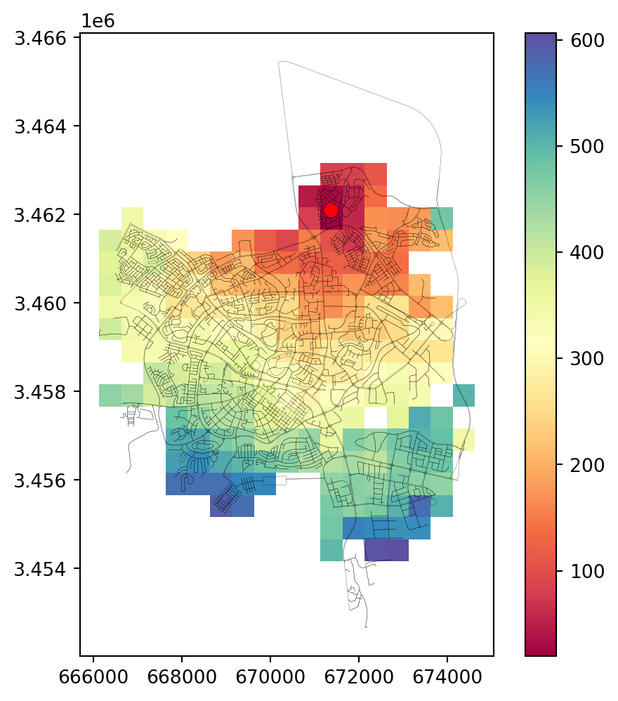
	geometry	time
0	POLYGON ((-250 4250, 0 4250, 0 ...	1442.773912
1	POLYGON ((-250 4000, 0 4000, 0 ...	1332.049276
2	POLYGON ((-250 3750, 0 3750, 0 ...	1266.698171
3	POLYGON ((-250 3500, 0 3500, 0 ...	1266.698171
4	POLYGON ((-250 3250, 0 3250, 0 ...	1332.049276
...	...	...
356	POLYGON ((4250 750, 4500 750, 4...	1165.238436
357	POLYGON ((4250 500, 4500 500, 4...	1131.923142
358	POLYGON ((4250 250, 4500 250, 4...	1126.274788
359	POLYGON ((4250 0, 4500 0, 4500 ...	1148.701574
360	POLYGON ((4250 -250, 4500 -250,...	1197.627331

361 rows × 2 columns

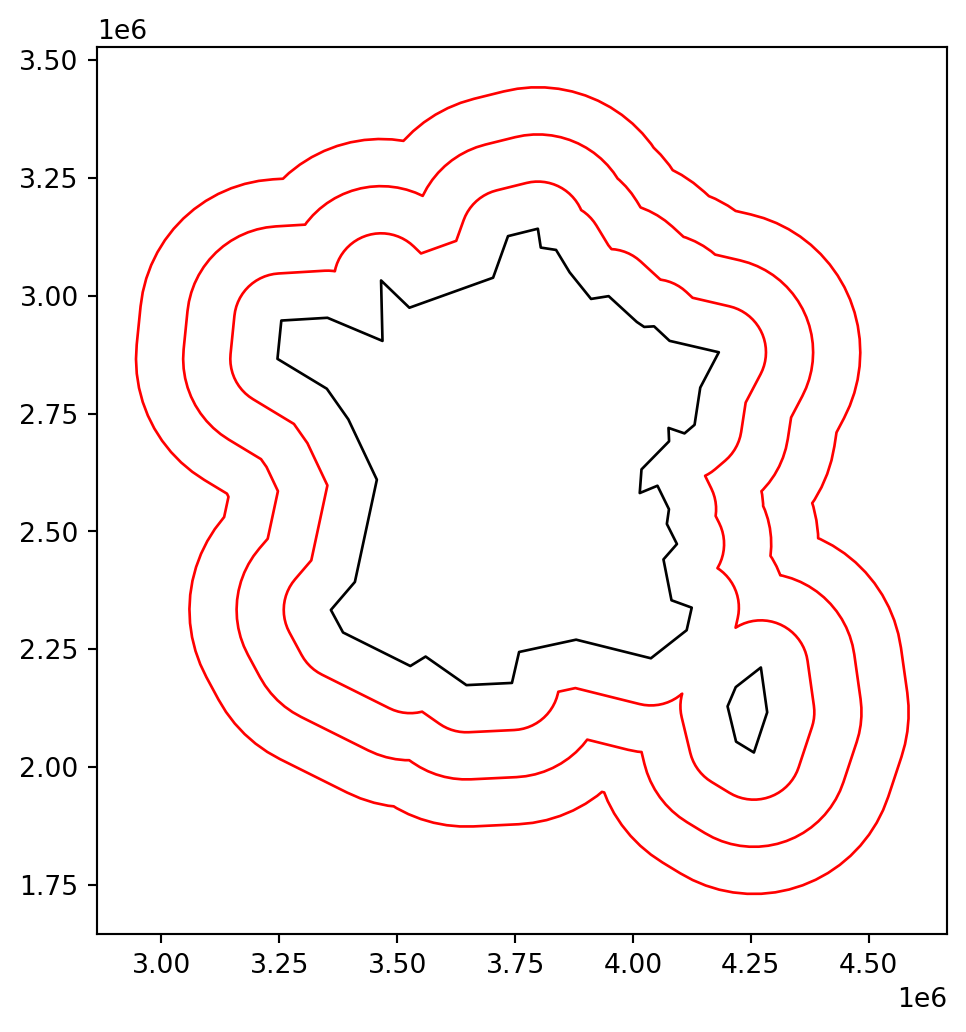
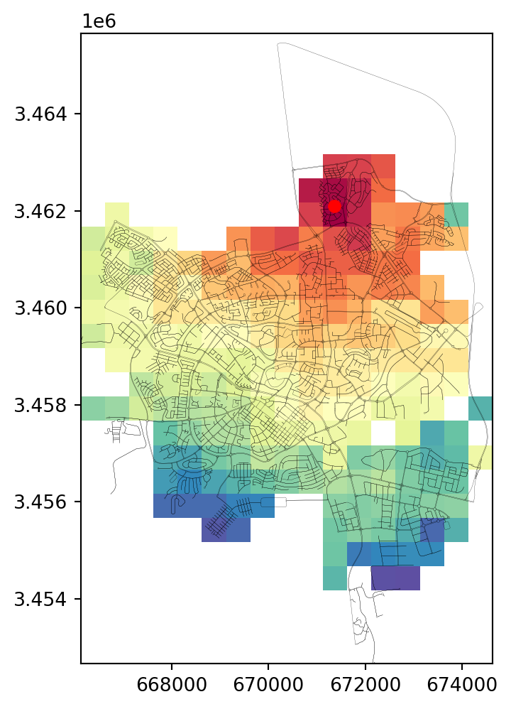
fig, ax = plt.subplots(figsize=(8, 5))
grid.plot(column='time', cmap='Spectral_r', legend=True, ax=ax)
nx.draw(G, pos=net2.pos(G), with_labels=True)
plt.plot(pnt.x, pnt.y, 'ro');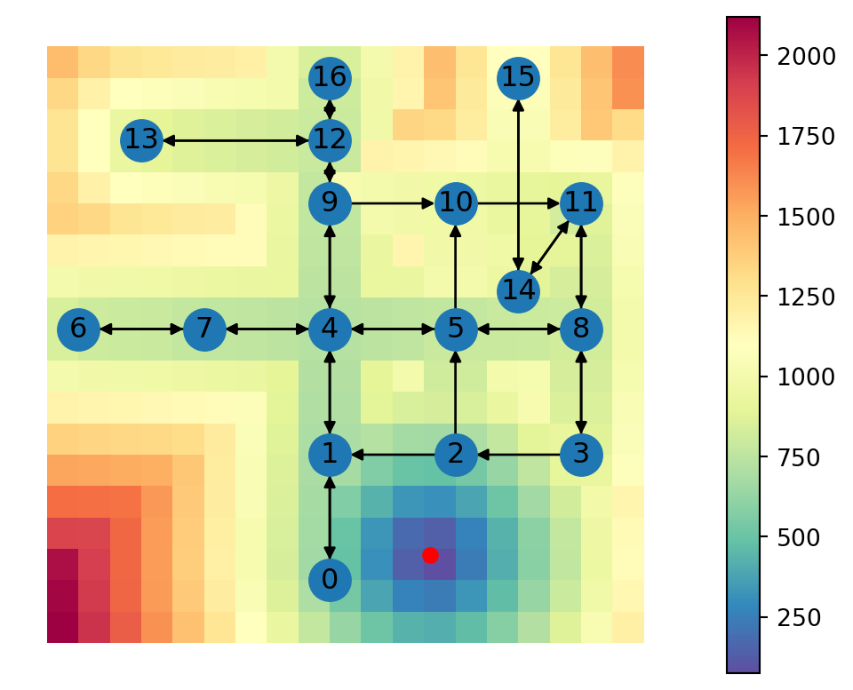

Figure 19.19: Travel time (\(sec\)) to a specific point (in red), on the modified single-component roads network

Solution 09-02

	geometry	mode
0	POLYGON ((-250 4250, 0 4250, 0 ...	walking+driving
1	POLYGON ((-250 4000, 0 4000, 0 ...	walking+driving
2	POLYGON ((-250 3750, 0 3750, 0 ...	walking+driving
3	POLYGON ((-250 3500, 0 3500, 0 ...	walking+driving
4	POLYGON ((-250 3250, 0 3250, 0 ...	walking+driving
...	...	...
356	POLYGON ((4250 750, 4500 750, 4...	walking
357	POLYGON ((4250 500, 4500 500, 4...	walking
358	POLYGON ((4250 250, 4500 250, 4...	walking
359	POLYGON ((4250 0, 4500 0, 4500 ...	walking
360	POLYGON ((4250 -250, 4500 -250,...	walking

361 rows × 2 columns

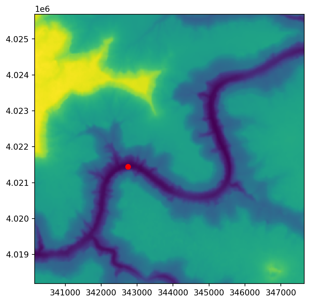
fig, ax = plt.subplots(figsize=(8, 5))
grid.plot(column='mode', cmap='Spectral_r', legend=True, ax=ax)
nx.draw(G, pos=net2.pos(G), with_labels=True)
plt.plot(pnt.x, pnt.y, 'ro');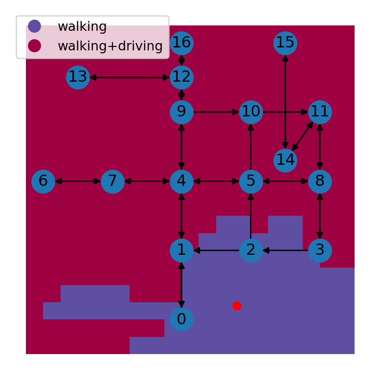

Figure 19.20: Optimal travel mode to a specific point (in red), on the modified single-component roads network

Solution 09-03

Figure 19.21: Travel time (\(sec\)) to a specific point (in black), on the modified single-component roads network, reclassified to discrete categories

Solution 10-01

Figure 19.22: Travel times to specific point in Beer-Sheva

Solution 10-02

import matplotlib.pyplot as plt
import pyproj
import shapely
import geopandas as gpd
import networkx as nx
import osmnx as ox
import net2

# Read network data
G = nx.read_graphml('output/beer-sheva.xml')
G = net2.prepare(G)

# Function definition
def find_route(G, orig, dest, crs):
    transformer = pyproj.Transformer.from_crs(4326, crs, always_xy=True)
    orig = ox.geocoder.geocode(orig)
    dest = ox.geocoder.geocode(dest)
    orig = shapely.Point(orig[1], orig[0])
    dest = shapely.Point(dest[1], dest[0])
    orig = shapely.transform(orig, transformer.transform, interleaved=False)
    dest = shapely.transform(dest, transformer.transform, interleaved=False)
    route = net2.route2(G, orig, dest, 'time')
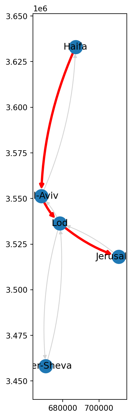
    return route

# Function call example
route = find_route(
    G, 
    'Turner Stadium, Beer-Sheva', 
    'Cinema City, Beer-Sheva', 
    32636
)
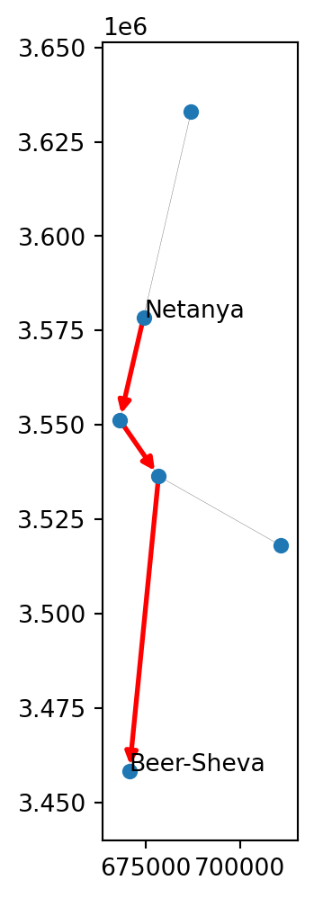
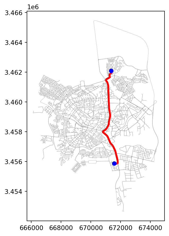
route['weight']

377.51506119393326

# Plot route
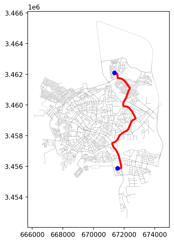
edges = net2.edges_to_gdf(route['network'])
route1 = net2.route_to_gdf(route['network'], route['route'])
base = edges.plot(color='grey', linewidth=0.2)
route1.plot(ax=base, color='red');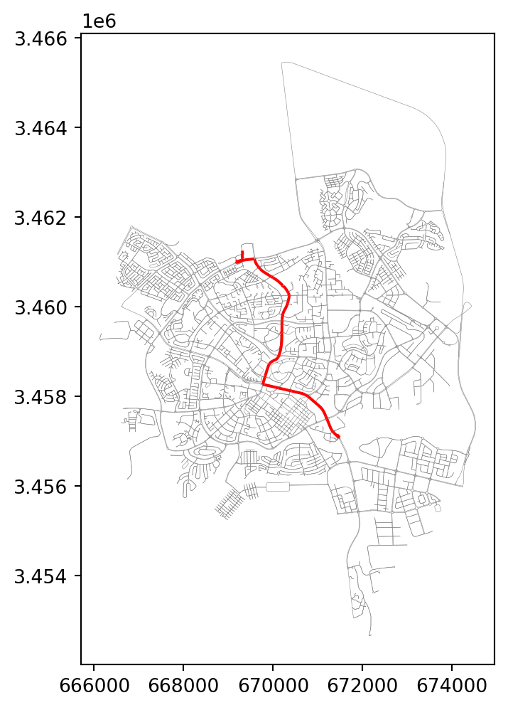

Figure 19.23: Fastest route from Turner Stadium to Cinema City, in Beer-Sheva

Solution 10-03

Figure 19.24: Travel time to specific point in Beer-Sheva

Figure 19.25: Travel time to specific point in Beer-Sheva, after modification of edge weights

Solution 11-01

Figure 19.26: ID of the nearest hospital in the Negev, with hypothetical third hospital in Mitzpe Ramon

Solution 11-02

Figure 19.27: Map of travel time matrix values (\(hr\)) between four locations in the Negev

Solution 11-03

Figure 19.28: Solution of the Traveling Salesman Problem for eight locations in the Negev

Solution 12-01

Figure 19.29: Two least cost paths through the Grand Canyon DEM

Solution 12-02

Figure 19.30: Travel time from specific point to all other points in the Grand Canyon DEM

Solution 12-03

Figure 19.31: Travel times to specific point in Beer-Sheva, in a raster-based grid representation

Solution 13-01

9205.547047891798

Solution 13-02

import fastapi

app = fastapi.FastAPI()

@app.get("/")
async def lonlat_to_utm(lon: float, lat: float):
    import math
    utm = (math.floor((lon + 180) / 6) % 60) + 1
    if lat > 0:
        utm += 32600
    else:
        utm += 32700
    return utm

Solution 13-03

Figure 19.32: Travel times to specific point in Beer-Sheva, calculated using a web API