Routing

Last updated: 2026-03-04 01:42:26

Introduction

In this chapter we introduce the central and most common task in spatial network analysis: finding the optinal route between two given points, also known as routing:

First, we show the basic usage of nx.shortest_path to find the optinal route between two points (Finding optimal route), and develop helper functions to calculate (Basic routing function) and graphically display (Graphics: Route) the calculated route.
We move on to examine the implications of choosing to minimize different types of weights—typically either distance or travel time in spatial networks (Choice of weights to minimize and Sum of route weights).
Next we demonstrate the effect of spatial network directions, namely the distinction between one-way or two-way road segments and its effects on routing (Effect of directions).
Finally, we cover the techniques to extract route edges along with their associated attributes (Route edges) and to transform them to a GeoSeries (Route to GeoDataFrame), which is useful when we need to apply further (non-network) spatial analysis techniques on the resulting route (such as evaluating which land use types it goes through, calculating an elevation profiles, etc.).

Packages

import matplotlib.pyplot as plt
import numpy as np
import pandas as pd
import shapely
import geopandas as gpd
import networkx as nx
import osmnx as ox
import net2

Sample data

To demonstrate routing, let’s start with the small road network in output/roads2.xml:

G = nx.read_graphml('output/roads2.xml')
G = net2.prepare(G)
G

<networkx.classes.digraph.DiGraph at 0x7698584e03e0>

To remind, we have 17 nodes:

G.nodes

NodeView((0, 1, 2, 3, 4, 5, 6, 7, 8, 9, 10, 11, 12, 13, 14, 15, 16))

And the edges are associated with 'geometry', 'length', 'speed', and 'time' attributes:

list(G.edges.data())[0]

(0,
 1,
 {'geometry': <LINESTRING (2000 0, 2000 1000)>,
  'length': 1000.0,
  'speed': 90,
  'time': 40.0})

Finding optimal route

The nx.shortest_path function can be used to calculate the shortest path between the specified nodes, given the attribute to minimize (weight). The result is a list of the nodes along the calculated path. The default optimal path search method of nx.shortest_path is Dijkstra’s algorithm.

For example, the following expression calculates the shortest route—i.e., the one with the minimum length—from node 3 to node 1:

route = nx.shortest_path(G, 3, 1, weight='length')
route

[3, 2, 1]

Graphics: Route

The nx.draw_networkx_edges function can be used to draw individual edges. That way, we can style some of the edges in a different way, e.g., when drawing a route along a network. Importantly, the nx.draw_networkx_edges function accepts an edgelist argument, which is a list of edges to draw.

For example, in Figure 8.1 we draw two specific edges—(4,5) and (12,13)—in red color (edge_color='r') and increased line width (width=3):

fig, ax = plt.subplots()
nx.draw(G, with_labels=True, pos=net2.pos(G), edge_color='grey', width=0.1, ax=ax)
nx.draw_networkx_edges(G, pos=net2.pos(G), edgelist=[(4,5),(12,13)], edge_color='r', width=3);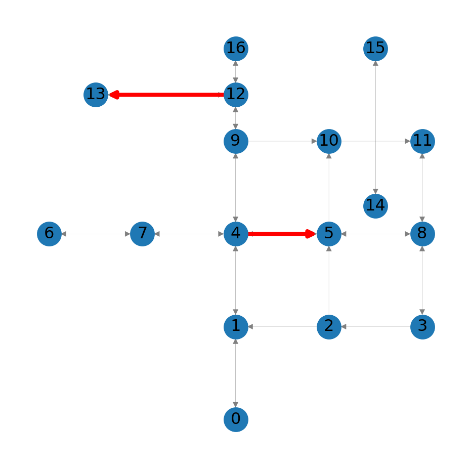

Figure 8.1: The road network with two specific edges drawn in red color

We are going to use the nx.draw_networkx_edges function to highlight the calculated route along the network. However, the route is defined through the nodes it goes through, rather than the edges:

route

[3, 2, 1]

To go from the nodes to edges, we use zip and indexing (zip):

list(zip(route, route[1:]))

[(3, 2), (2, 1)]

For example, Figure 8.2 highlights the route:

fig, ax = plt.subplots()
nx.draw(G, with_labels=True, pos=net2.pos(G), edge_color='grey', width=0.1, ax=ax)
nx.draw_networkx_edges(G, pos=net2.pos(G), edgelist=list(zip(route, route[1:])), edge_color='r', width=3);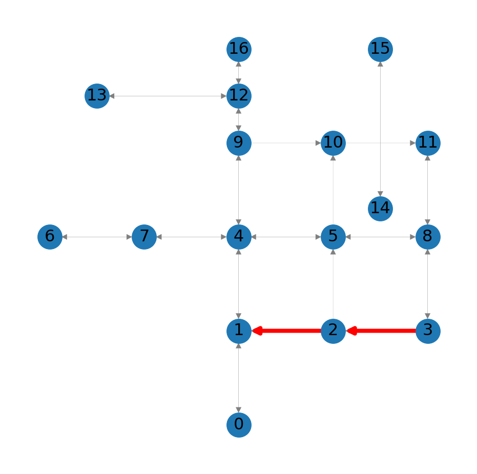

Figure 8.2: Shortest route from node `3` to node `1` in the roads network

Choice of weights to minimize

The weight parameter of the nx.shortest_path function lets us choose which edge weight to minimize when searching for the optimal route. For example, instead of the shortest route (weight='length'), we may want to search for the fastest route (weight='time'):

route2 = nx.shortest_path(G, 3, 1, weight='time')
route2

[3, 8, 5, 4, 1]

The fastest route (Figure 8.3) is not the same as the shortest route (Figure 8.2):

fig, ax = plt.subplots()
nx.draw(G, with_labels=True, pos=net2.pos(G), edge_color='grey', width=0.1, ax=ax)
nx.draw_networkx_edges(G, pos=net2.pos(G), edgelist=list(zip(route2, route2[1:])), edge_color='r', width=3);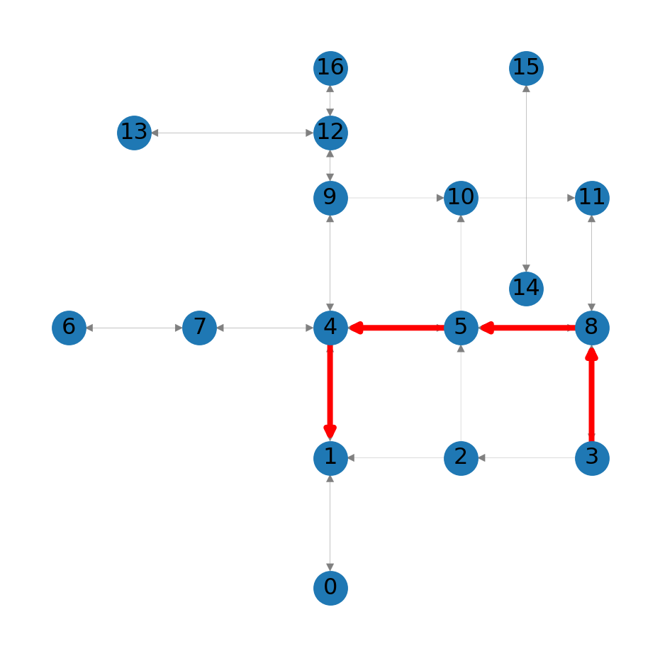

Figure 8.3: Fastest route from node `3` to node `1` in the roads network

Sum of route weights

The nx.path_weight function is used to calculate the sum of edge weights along the given route. For example, here we calculate the total length of route along G:

nx.path_weight(G, route, weight='length')

2000.0

In terms of length, we can see that route is shorter than route2:

nx.path_weight(G, route, weight='length'), nx.path_weight(G, route2, weight='length')

(2000.0, 4000.0)

However, in terms of time, we can see that route2 is faster:

nx.path_weight(G, route, weight='time'), nx.path_weight(G, route2, weight='time')

(240.00000000000003, 192.0)

Effect of directions

Note that routes can only follow edge directions. For example, the route from node 1 to adjacent node 2 has to go around because there is no direct 1→2 edge:

route = nx.shortest_path(G, 1, 2, weight='length')
route

[1, 4, 5, 8, 3, 2]

Practice

What happens if you omit the argument 2 from the above result?
Try to guess based on the result, and then check the documentation

A graphical illustration makes this more clear:

nx.draw(G, with_labels=True, pos=net2.pos(G), edge_color='grey', width=0.1)
nx.draw_networkx_edges(G, pos=net2.pos(G), edgelist=list(zip(route, route[1:])), edge_color='r', width=3);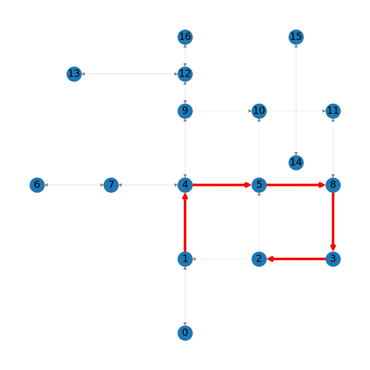

Figure 8.4: Shortest route from node `1` to node `2` in the roads network

Basic routing function

Let’s define a minimal routing function, named net2.route1:

def route1(network, node_start, node_end, weight):
    try:
        route = nx.shortest_path(network, node_start, node_end, weight)
        weight_sum = nx.path_weight(network, route, weight=weight)
        return {'route': route, 'weight': weight_sum}
    except:
        return {'route': np.nan, 'weight': np.nan}

The function accepts the network, start node, and end node. The additional parameter is the weight. The function then returns the route nodes, and the summed weight, calculated using nx.shortest_path and nx.path_weight, respectively, as shown above. For example:

net2.route1(G, 1, 2, 'length')

{'route': [1, 4, 5, 8, 3, 2], 'weight': 5000.0}

Note that the function has try/except code blocks. The interpreter tries to run the try block, and if an error is raised—then it runs the except block, where the function returns np.nan for the route and summed weight. For example, try finding the optimal route between nodes 14 and 1 with nx.shortest_path. You should see an error, because the nodes are disconnected:

nx.shortest_path(G, 14, 1, weight='length')

NetworkXNoPath: No path between 14 and 1.

Our net2.route1 function, however, does work:

net2.route1(G, 14, 2, 'length')

{'route': nan, 'weight': nan}

Route edges

The nx.path_graph function can be used to create a new network, consisting of consecutive edges along the list elements:

route_G = nx.path_graph(route)
route_G

<networkx.classes.graph.Graph at 0x7698581a6d80>

Figure 8.5 shows the result:

nx.draw(route_G, with_labels=True)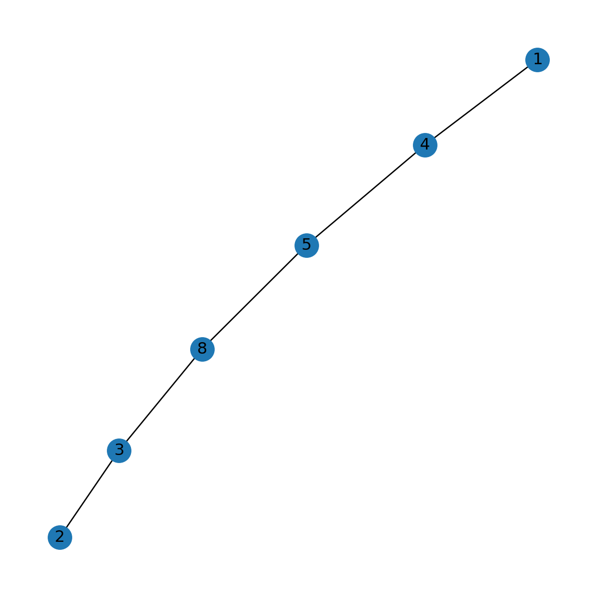

Figure 8.5: The route between nodes `1` and `2`, extracted to a sub-network object

Unfortunately, the data are lost:

route_edges = route_G.edges
dict(route_edges)

{(1, 4): {}, (4, 5): {}, (5, 8): {}, (8, 3): {}, (3, 2): {}}

In necessary, we can go over the respective edges in the original network G to get the attribute data, as follows:

for u,v in route_edges:
    x = G.edges[u,v]
    print(x)

{'geometry': <LINESTRING (2000 1000, 2000 2000)>, 'length': 1000.0, 'speed': 90, 'time': 40.0}
{'geometry': <LINESTRING (2000 2000, 3000 2000)>, 'length': 1000.0, 'speed': 90, 'time': 40.0}
{'geometry': <LINESTRING (3000 2000, 4000 2000)>, 'length': 1000.0, 'speed': 90, 'time': 40.0}
{'geometry': <LINESTRING (4000 1000, 4000 2000)>, 'length': 1000.0, 'speed': 50, 'time': 72.0}
{'geometry': <LINESTRING (3000 1000, 4000 1000)>, 'length': 1000.0, 'speed': 30, 'time': 120.00000000000001}

Route to `GeoDataFrame`

To create a line layer of the edges along a route, we can go over the edge properties and extract the 'geometry' attributes into a list:

geoms = [G.edges[u,v]['geometry'] for u,v in route_edges]
geoms

[<LINESTRING (2000 1000, 2000 2000)>,
 <LINESTRING (2000 2000, 3000 2000)>,
 <LINESTRING (3000 2000, 4000 2000)>,
 <LINESTRING (4000 1000, 4000 2000)>,
 <LINESTRING (3000 1000, 4000 1000)>]

Then, we can transform the list into a GeoSeries:

geom = gpd.GeoSeries(geoms)
geom

0    LINESTRING (2000 1000, 2000 2000)
1    LINESTRING (2000 2000, 3000 2000)
2    LINESTRING (3000 2000, 4000 2000)
3    LINESTRING (4000 1000, 4000 2000)
4    LINESTRING (3000 1000, 4000 1000)
dtype: geometry

Figure 8.6 shows the resulting line layer:

geom.plot(linewidth=5);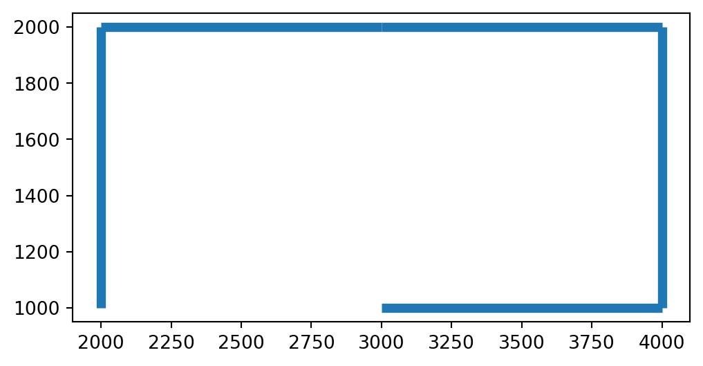

Figure 8.6: A `GeoDataFrame` representing a route through the network

When writing a function for the “route to GeoDataFrame” workflow, we must try to consider the possible edge cases, where the function may fail. For example, let’s see what happens when we try to find the route between an origin and a destination which are the same node?

route = nx.shortest_path(G, 1, 1, weight='length')
route

[1]

route_edges = nx.path_graph(route).edges
route_edges

EdgeView([])

The current workflow returns a \(0 \times 0\) GeoDataFrame:

result = []
for u,v in route_edges:
    x = G.edges[u,v]['geometry']
    result.append({'from': u, 'to': v, 'geometry': x})
result = gpd.GeoDataFrame(result)
result

result.shape

(0, 0)

It can be argued that it would make more sense returning a \(1 \times 3\) GeoDataFrame, with a “line” that goes from the origin to itself. That way, chances are improved that downstream processing of the result (such as displaying it on a map) will work:

result = []
pnt = G.nodes[route[0]]['geometry']
line = shapely.LineString([pnt, pnt])
print(line)

LINESTRING (2000 1000, 2000 1000)

result = gpd.GeoDataFrame([{'from': route[0], 'to': route[0], 'geometry': line}])
result

	from	to	geometry
0	1	1	LINESTRING (2000 1000, 2000 1000)

Incorporating both possible cases, the route_to_gdf function can be defined as follows:

def route_to_gdf(network, route, crs=None):
    route_edges = nx.path_graph(route).edges
    if len(route) == 1:
        result = []
        pnt = network.nodes[route[0]]['geometry']
        line = shapely.LineString([pnt, pnt])
        result = gpd.GeoDataFrame([{'from': route[0], 'to': route[0], 'geometry': line}], crs=crs)
    if len(route) > 1:
        result = []
        for u,v in route_edges:
            x = network.edges[u,v]['geometry']
            result.append({'from': u, 'to': v, 'geometry': x})
        result = gpd.GeoDataFrame(result, crs=crs)
    return result

Here is a demonstration of the function:

net2.route_to_gdf(G, route2)

	from	to	geometry
0	3	8	LINESTRING (4000 1000, 4000 2000)
1	8	5	LINESTRING (3000 2000, 4000 2000)
2	5	4	LINESTRING (2000 2000, 3000 2000)
3	4	1	LINESTRING (2000 1000, 2000 2000)

And here is a demonstration of the edge case:

net2.route_to_gdf(G, route)

	from	to	geometry
0	1	1	LINESTRING (2000 1000, 2000 1000)

Note

Routing in a road network can be further improved: * Adding penalty for junctions, assuming that there are traffic lights, or at least a “stop” or “give way” sign * Taking into account traffic, possibly from real-time data

Exercises

Exercise 07-01

Modify the roads network so that the 14,15 component is connected to the rest of the network in both directions. You can choose any way you like to connect the components: adding a new edge, adding new nodes, modifying existing edges, etc.
Make sure that the new edges and nodes (if any) contain all of the “standard” attributes that the other nodes and edges have (you can use any travel speed you like for the new edges)
Calculate and plot the fastest route from node 15 to node 7 (Figure 19.13)

Exercise 07-02

Re-create the directed railway network with time weights from Exercise 06-02
Calculate and plot the fastest route between Haifa and Jerusalem (Figure 19.14)
Calculate the total travel time along the route, and compare it to a manual sum of the segment travel times

Exercise 07-03

Calculate travel times from node 0 to all other nodes in the roads network. Mark unreachable nodes with -1.
Plot the network, displaying travel times on the edges, and the calculated travel times from node 0 for each node. Make node sizes proportional to the travel times from node 0 (Figure 19.15)

Introduction

Packages

Sample data

Finding optimal route

Graphics: Route

Choice of weights to minimize

Sum of route weights

Effect of directions

Basic routing function

Route edges

Route to GeoDataFrame

Exercises

Exercise 07-01

Exercise 07-02

Exercise 07-03

Route to `GeoDataFrame`