Last updated: 2026-03-04 01:42:09Networks with networkx
Introduction
In this chapter, we learn about the basics of working with spatial networks in Python, using package networkx:
We begin with introducing the concepts of spatial networks (What is a network?), the
networkxpackage (What is networkx?), and the data structures it provides for various types of networks (Network types in networkx)We move on to create a small network from scratch, for practice, while learning:
- how to create a network object (Creating network object),
- how to add nodes (Adding nodes),
- how to add edges (Adding edges), and
- how to remove nodes and edges (Removing nodes and edges)
We show how to export (Network to '.xml') and import (Network from '.xml')
networkxnetworks, to and from'.xml'files, respectively, for persistent storageWe introduce graphical display of networks to examine our data (Graphics: nx.draw, Graphics: node labels, Graphics: node size)
We learn about querying basic network properties, such as the number of nodes (Network properties)
We learn how to access specific nodes and edges (Accessing nodes and edges) and their associated attributes (Node attributes, Edge attributes). Furthermore, we show how to systematically go over all existing nodes and edges using iteration (Iteration over nodes and edges), which can be used to modify all network elements at once, or to locate specific elements.
We introduce the concept of network components (Components (undirected))
We learn how to transform and
networkxnetwork object into anndarray(packagenumpy) or into aDataFrame(packagepandas) (Network to numpy/pandas), and how to transform aDataFrameto anetworkxnetwork (Network from adjacency DataFrame)We cover three common metrics quantifying node importance: degree, degree centrality, and betweenness centrality (Node metrics)
Packages
import pandas as pd
import networkx as nx
What is a network?
A network, also known as a graph, is a set of nodes related through edges. For example, Figure 5.1 shows a network composed of:
- Four nodes (
A,B,C, andD) - Five edges (
A↔︎B,C↔︎D,A↔︎C,A↔︎D,B↔︎D)
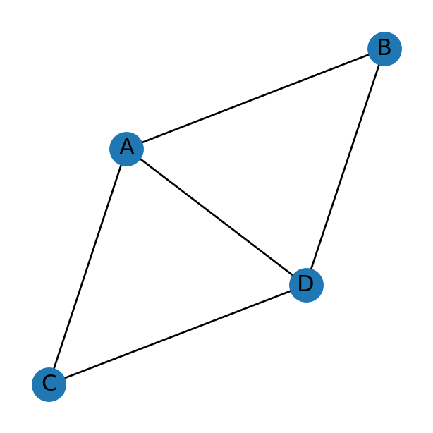
Note that the network does not necessarily contain all possible edges between the nodes. For example, there is no B↔︎C edge in the network depicted in Figure 5.1, implying that nodes B and C are unrelated.
Moreover, note that a network may contain isolated nodes (i.e., nodes which are not associated with any edges). A network can also be composed of more than one disconnected components. You can see an illustration of both cases in the network depicted in Figure 5.4, and in other examples throughout the book.
The basic type of information contained in a network is therefore two-fold:
- The list of nodes
- The list of edges
What is networkx?
Released in 2002, networkx (Hagberg, Schult, and Swart 2008) is an established package for network analysis in Python. It is currently the leading Python package in its category, with ~3 million daily downloads.
The networkx package contains functions to:
- create,
- modify,
- plot,
- import, and
- export
networks. The present chapter demonstrates the capabilities of networkx through examples.
Network types in networkx
The networkx package supports four types of networks (Table 5.1), represented through four specific classes, differing in terms of directionality ('Di') and possibility of parallel edges ('Multi'). Let’s define the latter two terms:
- A directed network has directed edges, i.e., edges whose direction matters
- A multi network is permitted to have parallel edges, i.e., more than one edge between the same pair of nodes (and in the same direction, if the network is directed)
networkx
| Class | Directed | Parallel edges | Example |
|---|---|---|---|
Graph |
| | Figure 5.2 |
DiGraph |
+ | | Figure 5.2 |
MultiGraph |
| + | |
MultiDiGraph |
+ | + | Figure 5.3 |
For example, Figure 5.1 depicts an undirected network. Accordingly, we see that there is (if any) just one edge between any given pair of nodes. Figure 5.2, however, depicts a directed network. Accordingly, we see that there may exist one or two (or zero) edges between any given pair of nodes, representing both possible directions. To distinguish the edge directions, they are drawn with arrowheads. The directed network depicted in Figure 5.2, for instance, has:
- Both of the two possible edges between nodes
AandB, i.e., bothA→BandB→A - One of the two possible edges between nodes
AandC, i.e., justA→C(but notC→A) - None of the two possible edges between nodes
BandC
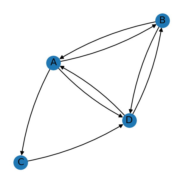
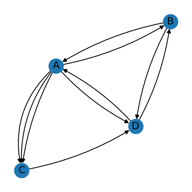
Figure 5.3 depicts a network that’s both directed and multi. The “multi” part means that there may be more than one edge of the same type, i.e., between the same two edges and having the same direction. In Figure 5.3, for instance, we can see that there are three A→C edges.
In practice, it is our job to choose the type of network which can represent the data we are working with. For example, a road network is typically directed, so that we have the ability to represent one-way streets. A road network may also have parallel edges, to have the ability to represent multiple road segments connecting begtween the same nodes (although for the practical purpose of routing, the network can be simplified by keeping just one “fastest” edge).
Creating network object
In networkx, a network is represented using a Graph object. When creating a network from scratch, we first create an empty Graph object with nx.Graph:
G = nx.Graph()
G
<networkx.classes.graph.Graph at 0x76cc8191bd10>Note that we’ve created undirected network without parallel edges (Table 5.1), which is the default. Later on in the book we will encounter other types of networks.
Adding nodes
Now, we can add nodes and edges. Nodes can be added using:
.add_node—Add one node.add_nodes_from—Add alistof nodes
For example, here we add one node representing the 'Asia' continent:
G.add_node('Asia')and here we’re adding multiple nodes for all other continents:
G.add_nodes_from([
    'Africa',
    'North America',
    'South America',
    'Antarctica',
    'Europe',
    'Australia'
])
Adding edges
Similarly, there are functions to add edges:
.add_edge—Add one edge.add_edges_from—add alistof edges
Note that each entry is of the form u,v, where u is the origin node and v is the destination node:
G.add_edge('Asia', 'Africa')
G.add_edges_from([['Asia', 'Europe'], ['North America', 'South America']])
Network to '.xml'
nx.write_graphml can be used to export a networkx network to a file in the GraphML format, for permanent storage. GraphML is a plain text XML-based file format for network data. It is supported by many network analysis programs (not just networkx).
For example, here we are exporting our network G to a file named 'continents.xml':
nx.write_graphml(G, 'output/continents1.xml')Here are the contents of the file 'continents.xml' we’ve just created. You can also open the file in a plain text editor to see for yourself:
<?xml version='1.0' encoding='utf-8'?>
<graphml xmlns="http://graphml.graphdrawing.org/xmlns" xmlns:xsi="http://www.w3.org/2001/XMLSchema-instance" xsi:schemaLocation="http://graphml.graphdrawing.org/xmlns http://graphml.graphdrawing.org/xmlns/1.0/graphml.xsd">
  <graph edgedefault="undirected">
    <node id="Asia" />
    <node id="Africa" />
    <node id="North America" />
    <node id="South America" />
    <node id="Antarctica" />
    <node id="Europe" />
    <node id="Australia" />
    <edge source="Asia" target="Africa" />
    <edge source="Asia" target="Europe" />
    <edge source="North America" target="South America" />
  </graph>
</graphml>
Network from '.xml'
We can import a network from an '.xml' file into the Python environment using nx.read_graphml:
G = nx.read_graphml('output/continents1.xml')
G
<networkx.classes.graph.Graph at 0x76cc81bfeba0>Graphics: nx.draw
The nx.draw function can be used to visualize a network object. In the resulting image, nodes are represented by points and edges are represented by lines. Using with_labels=True we choose to display node labels, which is a good idea for small networks (Figure 5.4):
nx.draw(G, with_labels=True)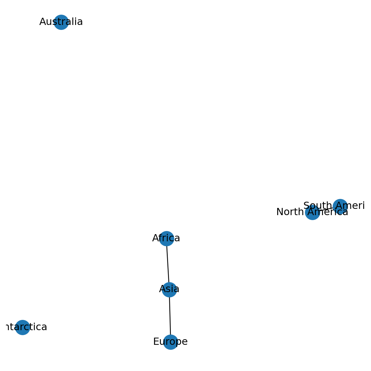
There are numerous other optional settings for nx.draw, some of which we will use in later chapters.
One important consideration is the placement of nodes in the plot two-dimensional space, also known as the “layout”. For a non-spatial network, the node positions are arbitrary; however, there are numerous authomatic algorithms for automatic placement. Many of the algorithms are random. For example, try re-running the above expression multiple times—you will see a different placement of the nodes each time!
Here is an example of another placing algorithm, called Kamada-Kawai. Using the nx.kamada_kawai_layout function, we first calculate a dict of node cooridinates, hereby named pos:
pos = nx.kamada_kawai_layout(G)
pos
{'Asia': array([ 0.4670448 , -0.06602379]),
'Africa': array([0.79648768, 0.86086687]),
'North America': array([-0.16834075, 1. ]),
'South America': array([-0.93747396, 0.38664351]),
'Antarctica': array([-0.88679401, -0.42707057]),
'Europe': array([ 0.11535165, -0.98489684]),
'Australia': array([ 0.61372461, -0.76951918])}The dictionary is then passed to the pos parameter of nx.draw:
nx.draw(G, with_labels=True, pos=pos)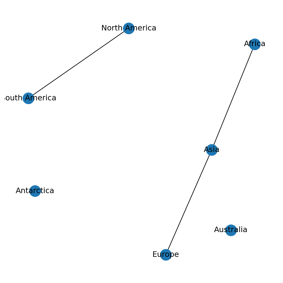
For a spatial network, the obvious layout is a “spatial” one, where the two-dimensional plot space represents geographic space, and node positions correspond to their spatial location. We will learn to use a spatial layout later on (Graphics: Spatial layout).
Removing nodes and edges
We can also remove existing nodes and edges from a network, which can be thought of as the opposite of adding them (see Adding nodes and Adding edges).
For example, a specific node can be removed with .remove_node:
G.remove_node('Asia')Figure 5.6 shows the resulting network. Note that removing a node also removes all edges connected to that node!
nx.draw(G, with_labels=True, pos=pos)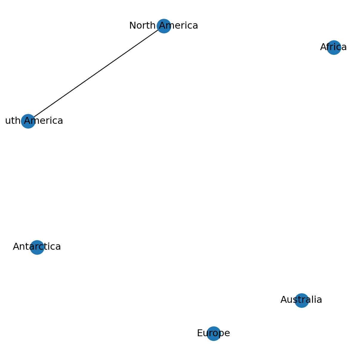
Similarly, a specific edge can be removed with .remove_edge:
G.remove_edge('North America', 'South America')Figure 5.7 shows the modified network:
nx.draw(G, with_labels=True, pos=pos)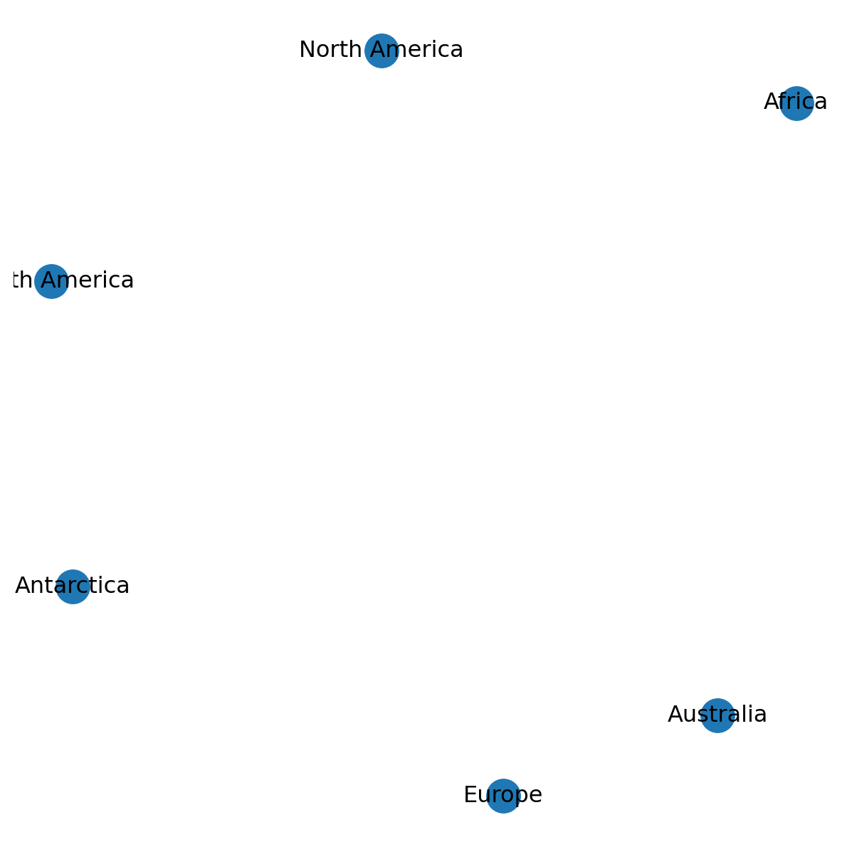
Let’s add the nodes and edges we removed to get back to the original network:
G.add_node('Asia')
G.add_edge('Asia', 'Europe')
G.add_edge('Asia', 'Africa')
G.add_edge('North America', 'South America')
Note that there are also methods remove_nodes_from and remove_edges_from, which are used to remove a list of nodes or edges, at once, respectively.
Network properties
Network size
The .number_of_nodes property returns the number of nodes in the given network:
G.number_of_nodes()7Similarly, .number_of_edges returns the number of edges:
G.number_of_edges()3Network .size is the total number of edges for an “unweghted” network (such as G in the following expression), or the sum of edge weights specified with weight='...' (see Network weights):
G.size()3Network type
The .is_directed property returns whether the network is directed (Network types in networkx):
G.is_directed()FalseThe .is_multigraph property returns whether the network is multi (Network types in networkx):
G.is_multigraph()FalseAccessing nodes and edges
Accessing nodes
The network nodes are accessible through the .nodes property:
G.nodesNodeView(('Africa', 'North America', 'South America', 'Antarctica', 'Europe', 'Australia', 'Asia'))If necessary, the nodes can be converted to a list or dict:
list(G.nodes)['Africa',
'North America',
'South America',
'Antarctica',
'Europe',
'Australia',
'Asia']dict(G.nodes){'Africa': {},
'North America': {},
'South America': {},
'Antarctica': {},
'Europe': {},
'Australia': {},
'Asia': {}}Accessing edges
Similarly, network edges can be accessed through .edges:
G.edgesEdgeView([('Africa', 'Asia'), ('North America', 'South America'), ('Europe', 'Asia')])which also can be convereted to a list or dict representation:
list(G.edges)[('Africa', 'Asia'), ('North America', 'South America'), ('Europe', 'Asia')]dict(G.edges){('Africa', 'Asia'): {},
('North America', 'South America'): {},
('Europe', 'Asia'): {}}Note that the edge IDs are tuples, where the elements are node IDs which the edge connects.
Note
Also see the Examining elements of a graph section in the networkx tutorial.
Node attributes
In the dict “view”, dictionary keys represent the nodes (e.g., 'Asia', 'Africa', etc.), while the dictionary values contain the node attributes, if any. Currently, the nodes in G have no attributes:
dict(G.nodes){'Africa': {},
'North America': {},
'South America': {},
'Antarctica': {},
'Europe': {},
'Australia': {},
'Asia': {}}Node attribuites can also be accessed directly, without going through dict:
G.nodes['Asia']{}G.nodesNodeView(('Africa', 'North America', 'South America', 'Antarctica', 'Europe', 'Australia', 'Asia'))We can set node attribute values using assignment:
G.nodes['Asia']['population'] = 4.85
G.nodes['Europe']['population'] = 0.75
Here are the updated node attributes of network G:
dict(G.nodes){'Africa': {},
'North America': {},
'South America': {},
'Antarctica': {},
'Europe': {'population': 0.75},
'Australia': {},
'Asia': {'population': 4.85}}
Note
Alternatively, we can use the nx.set_node_attributes function. This is more convenient when we want to set multiple attribute values at once, passed using a dict:
nx.set_node_attributes(G, {'Africa': {'x': 26.8, 'y': 1.3}})To delete an attribute, we can use del. For example, the following expression deletes the 'population' attribute of the 'Africa' node:
del G.nodes['Asia']['population']Here we can see the 'population' attribute was indeed deleted from 'Asia':
dict(G.nodes){'Africa': {},
'North America': {},
'South America': {},
'Antarctica': {},
'Europe': {'population': 0.75},
'Australia': {},
'Asia': {}}Edge attributes
The dict representation of edges contains the edge attributes:
dict(G.edges){('Africa', 'Asia'): {},
('North America', 'South America'): {},
('Europe', 'Asia'): {}}Specific edge attributes can also be accessed directly, as follows:
G.edges['Asia', 'Africa']{}Edge attributes can be set through assignment, similarly to node attributes:
G.edges['Asia', 'Africa']['distance'] = 5625Here is the modified network:
dict(G.edges){('Africa', 'Asia'): {'distance': 5625},
('North America', 'South America'): {},
('Europe', 'Asia'): {}}There is also a nx.get_edge_attributes, to get all values of a given attribute out of a network:
nx.get_edge_attributes(G, 'distance'){('Africa', 'Asia'): 5625}Deleting an edge attribute can be done using del, the same way as deleting a node attribute (see Node attributes).
Note
Also see the Adding attributes to graphs, nodes, and edges section in the networkx tutorial.
Iteration over nodes and edges
Sometimes we want to extract, or modify, the attributes of nodes or all edges, all at once. Using a for loop, we can go over G.nodes or G.edges, yielding the node or edge IDs, respectively:
for i in G.nodes:
    print(i)
Africa
North America
South America
Antarctica
Europe
Australia
Asiafor i in G.edges:
print(i)('Africa', 'Asia')
('North America', 'South America')
('Europe', 'Asia')Alternatively, when going over the edges, we can split the edge IDs straight into separate variables, conventinally named u and v:
for u,v in G.edges:
    print(u, '|', v)
Africa | Asia
North America | South America
Europe | AsiaInside the for loop, using the IDs, we can access the corresponding nodes or edges attributes:
for i in G.nodes:
    print(G.nodes[i])
{}
{}
{}
{}
{'population': 0.75}
{}
{}for u,v in G.edges:
print(G.edges[u, v]){'distance': 5625}
{}
{}Finally, we can make changes in the nodes or edges as part of the loop. For example, we can convert the 'population' attribute values of all nodes from int to str (after checking that it exists), as follows:
for i in G.nodes:
    if 'population' in G.nodes[i]:
        G.nodes[i]['population'] = str(G.nodes[i]['population'])
for i in G.nodes:
print(G.nodes[i]){}
{}
{}
{}
{'population': '0.75'}
{}
{}Components (undirected)
A components, in a network, is a sub-network where all nodes are reachable from each other. The number of components in an undirected network can be obtained with nx.number_connected_components:
nx.number_connected_components(G)4The list of nodes belonging to each component can be obtained with nx.connected_components:
list(nx.connected_components(G))[{'Africa', 'Asia', 'Europe'},
{'North America', 'South America'},
{'Antarctica'},
{'Australia'}]Isolated nodes
The nx.isolates function is used to detect isolated nodes, i.e., nodes that aren’t connected to anything through edges. The function returns a generator:
i = nx.isolates(G)
i
<generator object isolates.<locals>.<genexpr> at 0x76cc4bb47440>which, if necessary, can be converted to a list:
list(i)['Antarctica', 'Australia']Network to numpy/pandas
Network to ndarray (numpy)
The nx.to_numpy_array function can be used to transform a network to a numpy array. In the simplest case of an undirected network, and without specifying any particular weights, the result is a matrix where:
- Rows and columns represent nodes
- Cell values of
0or1represent absence or existence of an edge, respectively
For example:
nx.to_numpy_array(G)array([[0., 0., 0., 0., 0., 0., 1.],
[0., 0., 1., 0., 0., 0., 0.],
[0., 1., 0., 0., 0., 0., 0.],
[0., 0., 0., 0., 0., 0., 0.],
[0., 0., 0., 0., 0., 0., 1.],
[0., 0., 0., 0., 0., 0., 0.],
[1., 0., 0., 0., 1., 0., 0.]])Network to DataFrame (pandas)
nx.to_pandas_adjacency is similar to nx.to_numpy_array (Network to ndarray (numpy)), but returns a DataFrame rather than an array. Since a DataFrame has row and column names, we can also see the node IDs as part of the result:
nx.to_pandas_adjacency(G)| Africa | North America | South America | Antarctica | Europe | Australia | Asia | |
|---|---|---|---|---|---|---|---|
| Africa | 0.0 | 0.0 | 0.0 | 0.0 | 0.0 | 0.0 | 1.0 |
| North America | 0.0 | 0.0 | 1.0 | 0.0 | 0.0 | 0.0 | 0.0 |
| South America | 0.0 | 1.0 | 0.0 | 0.0 | 0.0 | 0.0 | 0.0 |
| ... | ... | ... | ... | ... | ... | ... | ... |
| Europe | 0.0 | 0.0 | 0.0 | 0.0 | 0.0 | 0.0 | 1.0 |
| Australia | 0.0 | 0.0 | 0.0 | 0.0 | 0.0 | 0.0 | 0.0 |
| Asia | 1.0 | 0.0 | 0.0 | 0.0 | 1.0 | 0.0 | 0.0 |
7 rows × 7 columns
nx.to_pandas_edgelist provides the transformation of a network to an “edge list”. The result is also a DataFrame, but instead of a pairwise matrix this is a list of all edges, including their source and target node IDs, as well as all attribute values (if any):
nx.to_pandas_edgelist(G)| source | target | distance | |
|---|---|---|---|
| 0 | Africa | Asia | 5625.0 |
| 1 | North America | South America | NaN |
| 2 | Europe | Asia | NaN |
Practice
What is the problem with this representation of network G?
Node metrics
Degree
The node degree is the number of edges adjacent to the node. The .degree property of a network returns the degrees of all nodes:
G.degreeDegreeView({'Africa': 1, 'North America': 1, 'South America': 1, 'Antarctica': 0, 'Europe': 1, 'Australia': 0, 'Asia': 2})The returned object can be transformed to a dict:
dict(G.degree){'Africa': 1,
'North America': 1,
'South America': 1,
'Antarctica': 0,
'Europe': 1,
'Australia': 0,
'Asia': 2}Degree centrality
The nx.degree_centrality function returns the Degree centrality of all nodes, which is the degree normalized by \(n-1\), where \(n\) is the number of nodes.
nx.degree_centrality(G){'Africa': 0.16666666666666666,
'North America': 0.16666666666666666,
'South America': 0.16666666666666666,
'Antarctica': 0.0,
'Europe': 0.16666666666666666,
'Australia': 0.0,
'Asia': 0.3333333333333333}degrees = dict(G.degree)
{key: degrees[key] / (G.number_of_nodes()-1) for key in degrees}{'Africa': 0.16666666666666666,
'North America': 0.16666666666666666,
'South America': 0.16666666666666666,
'Antarctica': 0.0,
'Europe': 0.16666666666666666,
'Australia': 0.0,
'Asia': 0.3333333333333333}Betweenness centrality
Betweenness centrality is a more elaborate measure of nodes centrality. Betweenness centrality is defined as the fraction of all-pairs shortest paths that pass through the given nodes. For example, in a road network, a node with higher betweenness centrality would be more important, because more volume of traffic will pass through that node.
The nx.betweenness_centrality function returns the betweenness centrality of the nodes:
bc = nx.betweenness_centrality(G)
bc
{'Africa': 0.0,
'North America': 0.0,
'South America': 0.0,
'Antarctica': 0.0,
'Europe': 0.0,
'Australia': 0.0,
'Asia': 0.06666666666666667}Graphics: node labels
As mentioned above (Graphics: nx.draw), using with_labels=True we can display node labels in a nx.draw plot. The default labels are the node IDs (e.g., Figure 5.7). Using the labels parameter, however, we can also specify any other, custom, node labels. The labels value has to be a dictionary of the form {node1:label1, node2:label2, ...}. For example, suppose we want to display the node degrees (Degree) as labels. The following object:
dict(G.degree){'Africa': 1,
'North America': 1,
'South America': 1,
'Antarctica': 0,
'Europe': 1,
'Australia': 0,
'Asia': 2}can be passed directly to the labels parameter, as follows (Figure 5.8):
nx.draw(G, with_labels=True, pos=pos, labels=dict(G.degree))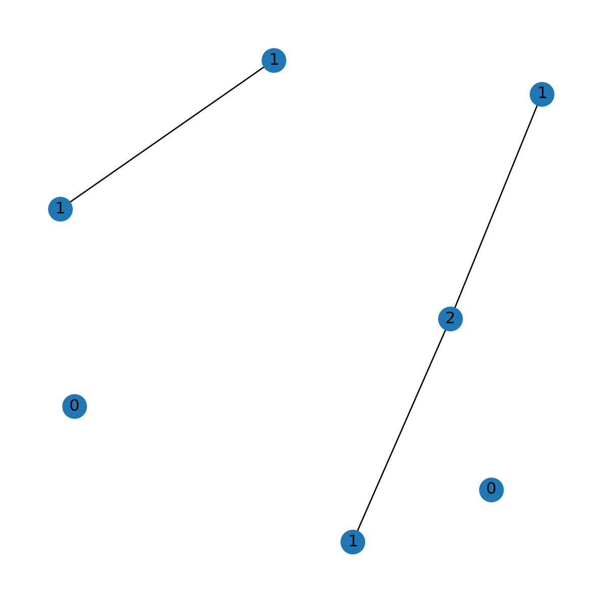
Graphics: node size
Node metrics can be visualized through variable node size, using the node_size parameter of nx.draw. For example, suppose that we want to visualize the node degree values (Degree):
v = dict(G.degree).values()
v
dict_values([1, 1, 1, 0, 1, 0, 2])The default in nx.draw is node_size=300. We can increase the values, through trial and error, until the plot (Figure 5.9) matches our needs. For example, here we use the arbitrary formula \(100+200\times v ^2\), where \(v\) are the degree values, so that the minimal node size is 300 and the maximal is 900:
v = [100+200*v**2 for v in v]
v
[300, 300, 300, 100, 300, 100, 900]Figure 5.9 shows the result, with node sizes porportional to their degrees:
nx.draw(G, with_labels=True, pos=pos, node_size=v)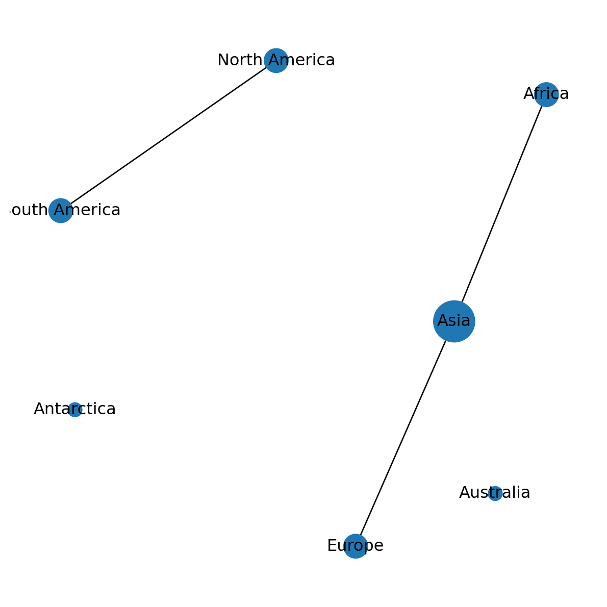
Network from adjacency DataFrame
A network can be created from an adjacency table. To demonstrate, let’s import the 'europe_borders.csv' table which we created in Pairwise matrices:
borders = pd.read_csv('output/europe_borders.csv', index_col=0)
borders| Albania | Austria | Belarus | Belgium | Bosnia and Herz. | ... | Sweden | Switzerland | Ukraine | United Kingdom | Russia | |
|---|---|---|---|---|---|---|---|---|---|---|---|
| Albania | True | False | False | False | False | ... | False | False | False | False | False |
| Austria | False | True | False | False | False | ... | False | True | False | False | False |
| Belarus | False | False | True | False | False | ... | False | False | True | False | True |
| ... | ... | ... | ... | ... | ... | ... | ... | ... | ... | ... | ... |
| Ukraine | False | False | True | False | False | ... | False | False | True | False | True |
| United Kingdom | False | False | False | False | False | ... | False | False | False | True | False |
| Russia | False | False | True | False | False | ... | False | False | True | False | True |
39 rows × 39 columns
The nx.from_pandas_adjacency function can transform a pairwise matrix, such as the one above, to a network object. This can be thought of as the reverse of nx.to_pandas_adjacency (Network to DataFrame (pandas)):
G = nx.from_pandas_adjacency(borders)
G
<networkx.classes.graph.Graph at 0x76cc4bbaa8a0>What we’ve created is a network where nodes represent European countries, and edges represent intersection, i.e., existence of a border between those countries. Figure 5.10 shows the result G graphically:
pos = nx.spring_layout(G, seed=100)
nx.draw(G, with_labels=True, pos=pos)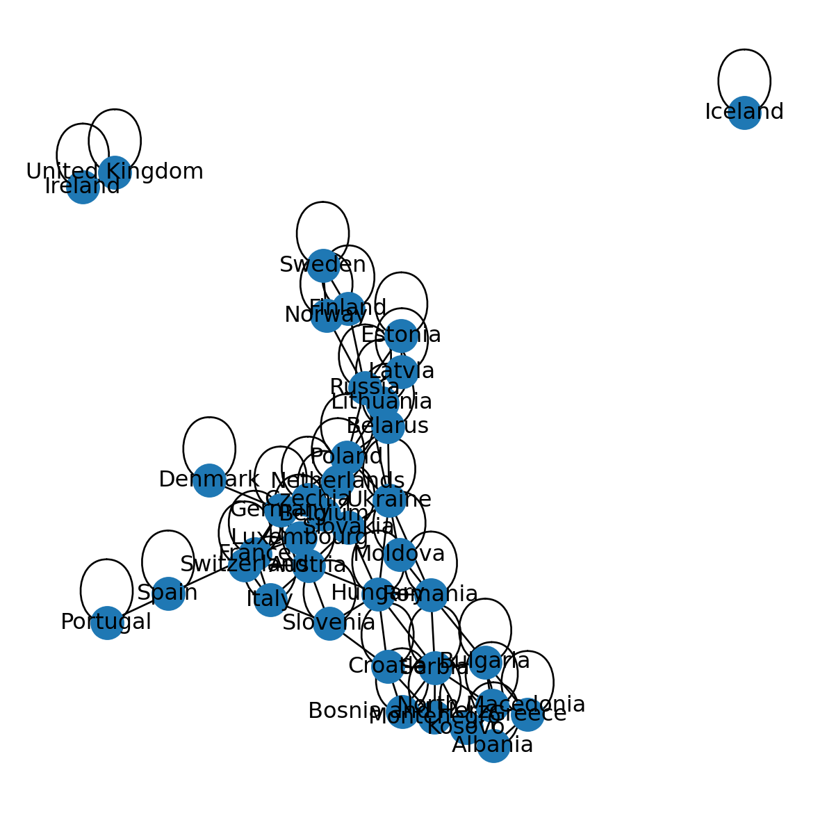
Note that the network contains edges going from a given node to itself. This type of edges is known as “self-loop” edges. In our present example G, in fact, all nodes are associated with self-loops, because the network represents shared intersection between countries, and every country intersects with itself. For example:
G.edges['Italy', 'Italy']{'weight': True}Self-loops can be removed using .remove_edges_from and nx.selfloop_edges, as follows:
G.remove_edges_from(nx.selfloop_edges(G))Figure 5.11 shows the modified network G, with self-loops removed. In plain language, the modified network G now represents shared borders between different countries:
nx.draw(G, with_labels=True, pos=pos)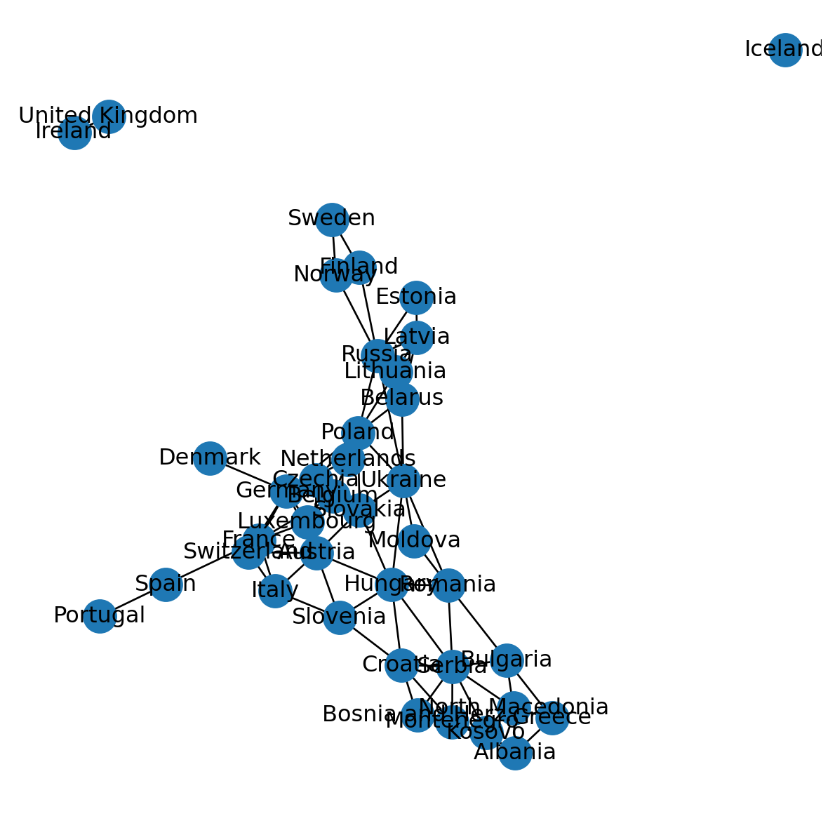
Exercises
Exercise 04-01
- Create a network representing the arrangement of students in the classroom where you are now:
- Nodes are students
- Edges can either represent students sharing the same desk or classroom row, or proximity (sitting on chairs next to each other)
- Plot the network (Figure 19.3)
Exercise 04-02
- Create a (partial) network representing railways between five cities in Israel
- Add the following nodes:
- Haifa
- Tel-Aviv
- Lod
- Jerusalem
- Beer-Sheva
- And the following edges:
- Haifa—Tel-Aviv
- Tel-Aviv—Lod
- Lod—Jerusalem
- Lod—Beer-Sheva
- Plot the network (Figure 19.4)
Exercise 04-03
- Re-create the European country borders network as shown in Network from adjacency DataFrame (Figure 5.11)
- Calculate the degree and the betweenness centrality of European countries
- Which country has the highest degree, and what is the degree value?
- Which country has the highest betweenness centrality, and what is the betweenness centrality value?
- Calculate the number of components in the Europe borders network
- Add two new edges which connect the components, then repeat the calculation to demonstrate that the number of components is now
1 - Plot the modified network (Figure 19.5)