Last updated: 2026-03-04 01:42:20Directions and weights
Introduction
In this chapter we introduce the concepts of directions and weights in spatial networks.
Spatial networks are typically directed. For example, road segments in both directions may differ in terms of travel time, or one of the directions may even not exist (e.g., one-way street).
Weights in spatial network edges typically convey information about distance and travel time, which is subsequently used in routing.
To get familiar with the concepts of directions and weights, we go through the following milestones:
We create a directed network of continents, from scratch (Creating directed network), illustrating the difference from the undirected continents network we previously created (Node 'geometry')
We then go back to the road network example, and make it directed as well (Transforming to directed)
We move on to introduce network weights. First, we access existing weights of distance (length) (Network weights). Second, we add travel speed weights (Adding travel speeds). Third, taking into account distance and travel speed, we calculate travel time weights (Calculating travel times).
Finally, we illustrate the concept of network components, now with a directed network (Components (directed))
Packages
import pandas as pd
import shapely
import geopandas as gpd
import networkx as nx
import osmnx as ox
import net2
Creating directed network
In a directed network, the direction of edges matters: edge A→B and edge B→A are two different possible edges between nodes A and B (unlike an undirected network, where there is one possible edge A↔︎B). As an example of creating a directed network from scratch, we will re-create the continents spatial network (Figure 6.6), but this time as a directed network.
In the directed continents network, edges are going to represent the directions of early human migration.
First, we create a new network object G using nx.DiGraph:
G = nx.DiGraph()
G
<networkx.classes.digraph.DiGraph at 0x7ace30115700>We add the continent nodes exactly the same way as when creating an undirectional network:
G.add_nodes_from([
    'Asia',
    'Africa',
    'North America',
    'South America',
    'Antarctica',
    'Europe',
    'Australia'
])
G.nodes['Africa']       ['geometry'] = shapely.Point(26.8, 1.3)
G.nodes['Asia']         ['geometry'] = shapely.Point(73.1, 39.5)
G.nodes['Australia']    ['geometry'] = shapely.Point(133.1, -24.9)
G.nodes['North America']['geometry'] = shapely.Point(-99.9, 39.6 )
G.nodes['South America']['geometry'] = shapely.Point(-55.4, -20.7)
G.nodes['Europe']       ['geometry'] = shapely.Point(34.3, 53.6 )
G.nodes['Antarctica']   ['geometry'] = shapely.Point(69.0, -76.1)
The code for creating the edges appears similar. However, inthe case of a directed network, the order of the nodes comprising the egde matters. For example, 'Africa','Asia' implies the 'Africa'→'Asia' edges. We could create an 'Asia'→'Africa' edge, which would be an independent separate edge:
G.add_edges_from([
    ('Africa', 'Asia'),
    ('Asia', 'Europe'),
    ('Asia', 'Australia'),
    ('Asia', 'North America'),
    ('North America', 'South America')
])
Let’s also import the country polygons to draw the network on a map:
d = gpd.read_file('data/ne_110m_admin_0_countries.shp')And here is the code for the map (Figure 7.1):
base = d.plot(color='none', edgecolor='lightgrey')
nx.draw(G, pos=net2.pos(G), ax=base, with_labels=True);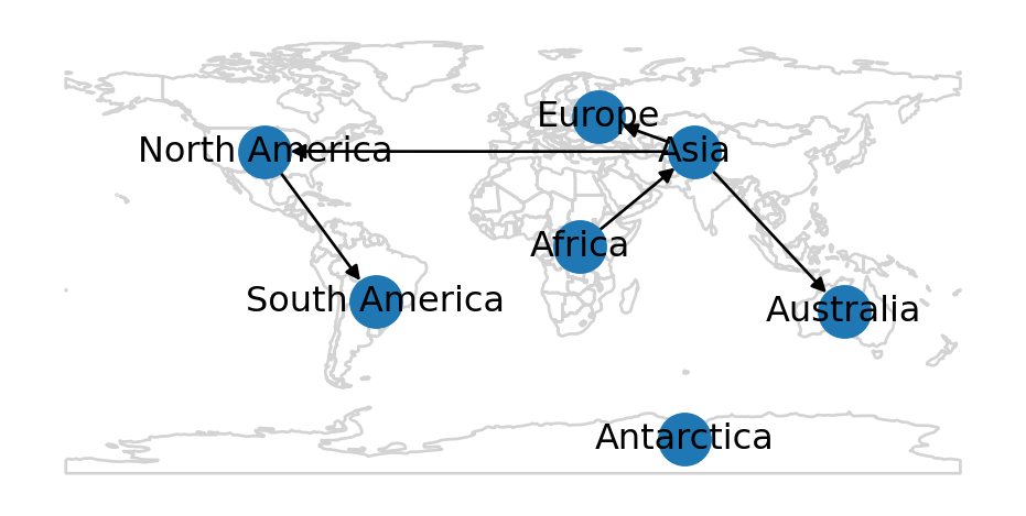
Sample data
In the subsequent examples in this chapter, we are going to work with the roads network (Sample data 2). First, let’s import it from the 'roads.xml' file:
G = nx.read_graphml('data/roads.xml')
G
<networkx.classes.graph.Graph at 0x7acd7250cfe0>Next, as explained earlier (Preparing a spatial network), we need to prepare and standardize the spatial network:
G = net2.prepare(G)
G
<networkx.classes.graph.Graph at 0x7acdb26e0590>Let’s examine the attributes of one node and one edge, for example:
G.nodes[list(G.nodes)[0]]{'geometry': <POINT (2000 0)>}G.edges[list(G.edges)[0]]{'geometry': <LINESTRING (2000 0, 2000 1000)>, 'length': 1000.0}And here is a plot of the network (Figure 7.2):
nx.draw(G, with_labels=True, pos=net2.pos(G))
roads.xml
In the following sections, we are going to implement directionality (Transforming to directed) and travel time weights (Calculating travel times). These two properties are going to be essential for network routing, as we will see in later chapters (Routing).
Transforming to directed
An existing network object can be transformed to a directed network using the .to_directed method. Note that the network type changes from Graph to DiGraph (Table 5.1):
G = G.to_directed()
G
<networkx.classes.digraph.DiGraph at 0x7acdb26ba120>As part of the conversion to DiGraph, each edge (u,v,data) is replaced by two edges (u,v,data) and (v,u,data). The fact that the network is now directed is also reflected in the plot, where edges are shown with arrowheads:
nx.draw(G, with_labels=True, pos=net2.pos(G))
DiGraph
In a road network, two-way streets are represented by edges in both directions, while one-way streets are represented by edges in one direction only. To make some of the road segments in the network G one-way, we are going to delete some of the edges:
G.remove_edge(11, 10)
G.remove_edge(10, 9)
G.remove_edge(10, 5)
G.remove_edge(5, 2)
G.remove_edge(1, 2)
G.remove_edge(2, 3)
The result is shown in Figure 7.4. Note how some of the road segments are now one way (e.g., 2→3).
nx.draw(G, with_labels=True, pos=net2.pos(G))
Graphics: Edges as arcs
Using connectionstyle='arc3,rad=0.1' we can display the edges as arcs, making the difference between one-way and two-way road segments more evident (Figure 7.5):
nx.draw(G, with_labels=True, pos=net2.pos(G), connectionstyle='arc3,rad=0.1')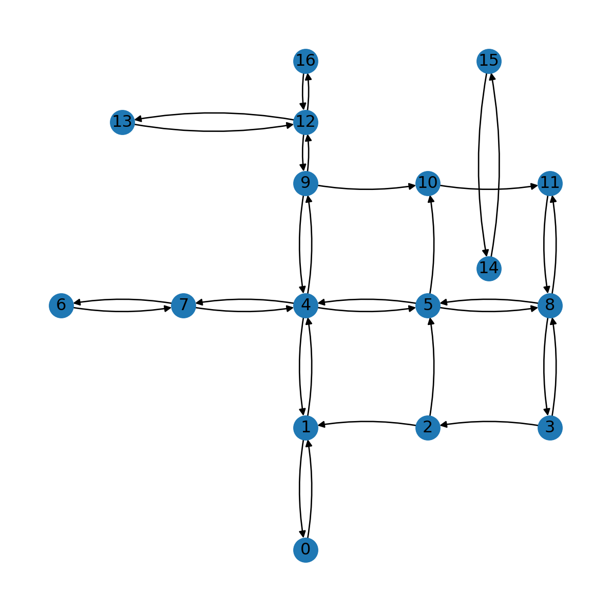
Degree (directed)
Node degree is the number of edges associated with the node (Figure 7.6). In a directed network, this includes edges in both directions, i.e., where the given node is either the origin or the destination.
For example, here are the node degrees in the directed road network G:
G.degreeDiDegreeView({0: 2, 1: 5, 2: 3, 3: 3, 4: 8, 5: 6, 6: 2, 7: 4, 8: 6, 9: 5, 10: 3, 11: 3, 12: 6, 13: 2, 14: 2, 15: 2, 16: 2})And here they are transformed to dict:
d = dict(G.degree)
d
{0: 2,
1: 5,
2: 3,
3: 3,
4: 8,
5: 6,
6: 2,
7: 4,
8: 6,
9: 5,
10: 3,
11: 3,
12: 6,
13: 2,
14: 2,
15: 2,
16: 2}Figure Figure 7.6 shows the node degrees:
nx.draw(G, pos=net2.pos(G), node_size=[v * 100 for v in d.values()], connectionstyle='arc3,rad=0.1')
nx.draw_networkx_labels(G, pos=net2.pos(G), labels={n: d[n] for n in G});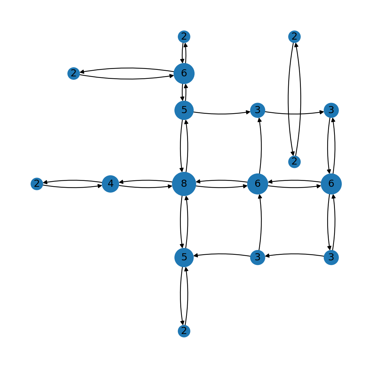
Network weights
Edge attributes can participate in network analysis algorithms, in which case they are known as weights. For example, shortest path algorithms can be used to calculate the optimal path between given nodes while minimizing the total edge weights (Finding optimal route).
For example, the edges in the roads network G are associated with an attribute named 'length', which represents the edge length in \(m\). The 'length' attribute can be used as network weights when calculating the shortest path between given nodes (Finding optimal route). Using nx.get_edge_attributes (Edge attributes) we can extract all of the edge lengths into a dict named weights:
weights = nx.get_edge_attributes(G, 'length')
weights
{(0, 1): 1000.0,
(1, 0): 1000.0,
(1, 4): 1000.0,
(2, 1): 1000.0,
(2, 5): 1000.0,
(3, 2): 1000.0,
(3, 8): 1000.0,
(4, 1): 1000.0,
(4, 7): 1000.0,
(4, 5): 1000.0,
(4, 9): 1000.0,
(5, 4): 1000.0,
(5, 8): 1000.0,
(5, 10): 1000.0,
(6, 7): 1000.0,
(7, 4): 1000.0,
(7, 6): 1000.0,
(8, 3): 1000.0,
(8, 5): 1000.0,
(8, 11): 1000.0,
(9, 4): 1000.0,
(9, 10): 1000.0,
(9, 12): 500.0,
(10, 11): 1000.0,
(11, 8): 1000.0,
(12, 9): 500.0,
(12, 13): 1500.0,
(12, 16): 500.0,
(13, 12): 1500.0,
(14, 15): 1700.0,
(15, 14): 1700.0,
(16, 12): 500.0}Graphics: Edge labels
The nx.draw_networkx_edge_labels function can be used to draw labels with the weights on top of edge line segments. Before applying it, let’s transform the weights from float to int, so that the label will be shorter:
labels = weights.copy()
for i in labels:
    labels[i] = int(labels[i])
labels
{(0, 1): 1000,
(1, 0): 1000,
(1, 4): 1000,
(2, 1): 1000,
(2, 5): 1000,
(3, 2): 1000,
(3, 8): 1000,
(4, 1): 1000,
(4, 7): 1000,
(4, 5): 1000,
(4, 9): 1000,
(5, 4): 1000,
(5, 8): 1000,
(5, 10): 1000,
(6, 7): 1000,
(7, 4): 1000,
(7, 6): 1000,
(8, 3): 1000,
(8, 5): 1000,
(8, 11): 1000,
(9, 4): 1000,
(9, 10): 1000,
(9, 12): 500,
(10, 11): 1000,
(11, 8): 1000,
(12, 9): 500,
(12, 13): 1500,
(12, 16): 500,
(13, 12): 1500,
(14, 15): 1700,
(15, 14): 1700,
(16, 12): 500}Now the dict can be passed to nx.draw_networkx_edge_labels, along with the network object and node positions, as follows (Figure 7.7):
nx.draw(G, with_labels=True, pos=net2.pos(G))
nx.draw_networkx_edge_labels(G, net2.pos(G), labels);
The 'connectionstyle' parameter can be used to for elliptical arcs, so that we can see the properties of edges in both directions:
nx.draw(G, with_labels=True, pos=net2.pos(G), connectionstyle='arc3,rad=0.15')
nx.draw_networkx_edge_labels(G, net2.pos(G), labels, connectionstyle='arc3,rad=0.15');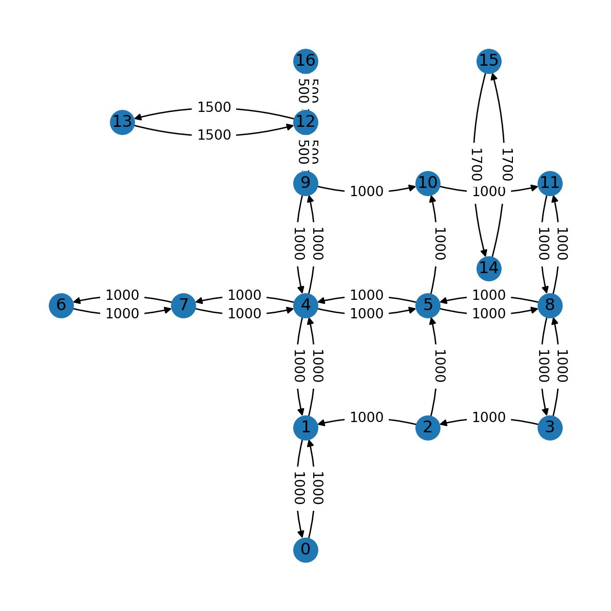
Adding travel speeds
When finding the optimal path on a road network, we are typically interested in the fastest rather than the shortest route. To be able to calculate the fastest route we need to have travel time edge weights. To have those, let’s add driving speeds to the edges. In terms of code, note how we set 90 (\(km\)/\(hr\)) on all edges, then replace the speed with 50 and 30 for some of the road segments:
nx.set_edge_attributes(G, {i:90 for i in list(G.edges)}, 'speed')
nx.set_edge_attributes(G,  {
    (2, 1): 30,
    (2, 5): 30,
    (3, 2): 30,
    (3, 8): 50,
    (5, 10): 50,
    (8, 3): 50,
    (8, 11): 50,
    (9, 10): 50,
    (10, 11): 50,
    (11, 8): 50,
    (12, 13): 50,
    (13, 12): 50,
    (14, 15): 50,
    (15, 14): 50
}, 'speed')
G
<networkx.classes.digraph.DiGraph at 0x7acdb26ba120>Figure 7.9 shows the road segments speeds we just added:
nx.draw(G, with_labels=True, pos=net2.pos(G))
edge_labels = nx.get_edge_attributes(G, 'speed')
nx.draw_networkx_edge_labels(G, net2.pos(G), edge_labels);
Graphics: Edge line widths
To highlight the different speeds of the road segments, we can use the width argument of nx.draw to draw edges with different line widths. First, we extract the speeds to an array and standardize them so that edges with 30 are displayed with the default line width (weight=1.0), while speeds of 60 or 90 are shown with double or triple line widths, respectively:
weights = [G[u][v]['speed']/30 for u,v in G.edges]
weights[:5]
[3.0, 3.0, 3.0, 1.0, 1.0]Then, the array is passed to the width parameter of nx.draw (Figure 7.10):
nx.draw(G, with_labels=True, pos=net2.pos(G), width=weights)
edge_labels = nx.get_edge_attributes(G, 'speed')
nx.draw_networkx_edge_labels(G, net2.pos(G), edge_labels);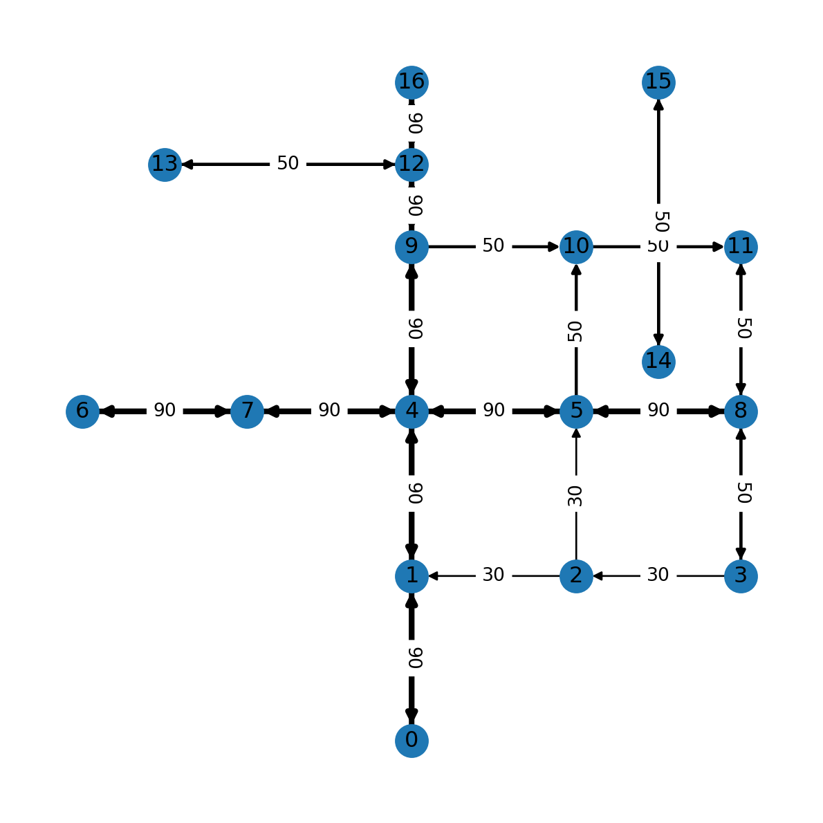
Calculating travel times
Now that every edge has length and speed attributes, we can also calculate time (travel time) attributes, which are essential for routing calculations:
G.edges[list(G.edges)[0]]{'geometry': <LINESTRING (2000 0, 2000 1000)>, 'length': 1000.0, 'speed': 90}We consider road lengths to be in \(m\), and speeds—in \(km/hr\). Therefore, we calculate time in \(sec\) using Equation 7.1:
\[ time (sec) = \frac{length(m)}{speed(km/hr) \times \frac{1000}{60 \times 60}} = \frac{length(m)}{speed(km/hr)} \times 3.6 \tag{7.1}\]
Here is the code to add travel times, in \(sec\), to the edge attributes. Note that for simplicity we also round the times to the nearest second:
for u,v in G.edges:
    G[u][v]['time'] = (G[u][v]['length'] / G[u][v]['speed']) * 3.6
    # G[u][v]['time'] = round(G[u][v]['time'])
Now, every edge also has a time attribute:
dict(G.edges)[0,1]{'geometry': <LINESTRING (2000 0, 2000 1000)>,
'length': 1000.0,
'speed': 90,
'time': 40.0}For plotting, we may want to round the 'time' attribute values:
edge_labels = nx.get_edge_attributes(G, 'time')
edge_labels = {key: round(value) for key,value in edge_labels.items()}
edge_labels
{(0, 1): 40,
(1, 0): 40,
(1, 4): 40,
(2, 1): 120,
(2, 5): 120,
(3, 2): 120,
(3, 8): 72,
(4, 1): 40,
(4, 7): 40,
(4, 5): 40,
(4, 9): 40,
(5, 4): 40,
(5, 8): 40,
(5, 10): 72,
(6, 7): 40,
(7, 4): 40,
(7, 6): 40,
(8, 3): 72,
(8, 5): 40,
(8, 11): 72,
(9, 4): 40,
(9, 10): 72,
(9, 12): 20,
(10, 11): 72,
(11, 8): 72,
(12, 9): 20,
(12, 13): 108,
(12, 16): 20,
(13, 12): 108,
(14, 15): 122,
(15, 14): 122,
(16, 12): 20}Figure 7.11 shows the travel times we calculated per road segment:
nx.draw(G, with_labels=True, pos=net2.pos(G))
nx.draw_networkx_edge_labels(G, net2.pos(G), edge_labels);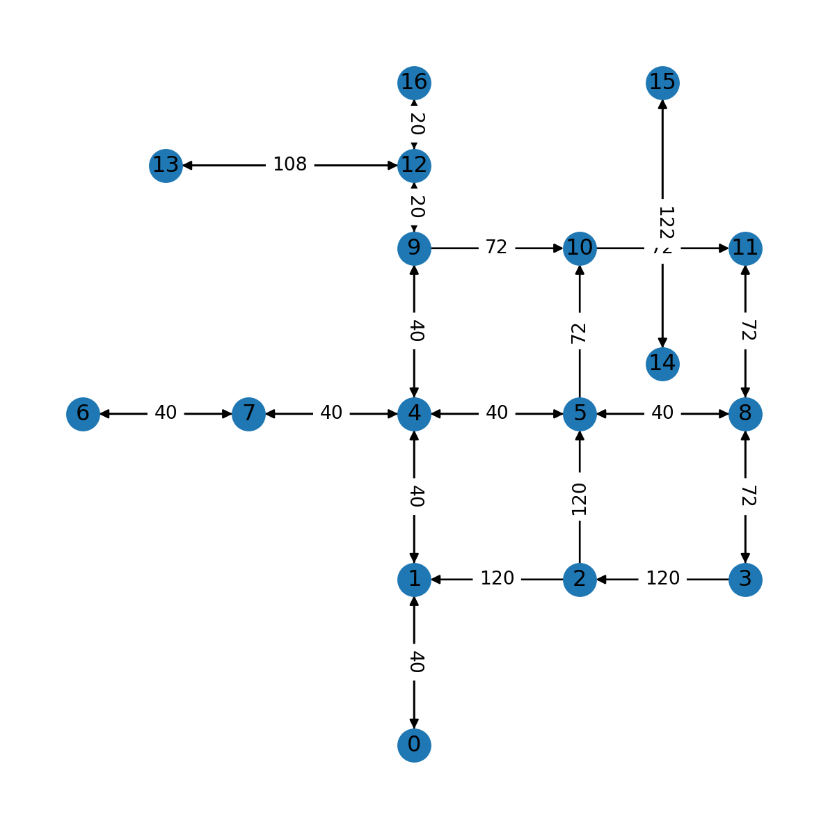
Writing 'roads2.xml'
Let’s export the modified (directional and weighted) road network to a new file named 'roads2.xml'. Before we do that, we need to transform the edge geometries to strings (Spatial network to '.xml'):
for i in G.nodes:
    G.nodes[i]['geometry'] = str(G.nodes[i]['geometry'])
for u,v in G.edges:
    G[u][v]['geometry'] = str((G[u][v]['geometry']))
nx.write_graphml_xml(G, 'output/roads2.xml')
Components (directed)
Earlier (Components (undirected)), we defined the concept of components for an undirected graph. In a directed network, two types of components are distinguished:
- Strongly connected—where every node is reachable from every other node
- Weakly connected—where every node is reachable from every other node when ignoring directions
The number of strongly connected components is obtained with nx.number_strongly_connected_components:
nx.number_strongly_connected_components(G)2The list of nodes belonging to each component can be obtained with nx.strongly_connected_components:
list(nx.strongly_connected_components(G))[{0, 1, 2, 3, 4, 5, 6, 7, 8, 9, 10, 11, 12, 13, 16}, {14, 15}]Exercises
Exercise 06-01
- Create a directed spatial network:
- with four nodes,
- where the nodes are arranged as if they are the corners of a rectangle which isn’t a square, and
- there are four edges which are the sides of the rectangle, along the “clockwise” direction
- Calculate the edge geometries
- Calculate the
'length'weights - Draw a spatial plot of the network with edge weight labels (Figure 19.10)
Exercise 06-02
- Recreate the rail network from Exercise 05-02
- Transform the network into a directed one
- Add segment geometries to the network, assuming the edges are straight line segments
- Transform the geometries to a projected CRS (
EPSG:32636) - Calculate edge
'length'attributes (in \(km\)), based on the geometries - Calculate edge
'time'(i.e., travel time, in \(hr\)) attributes, assuming that travel speed is 100 \(km/hr\) - Plot the network, with “time” labels on top of the edges (Figure 19.11)
Exercise 06-03
- The following code defines a
DataFramerepresenting amount of Tomatoes traded between three European countries, in tonnes, in 2020:
dat = pd.DataFrame({
    'origin': ['France','France','Spain','Spain','Italy','Italy'],
    'destination': ['Spain','Italy','Italy','France','Spain','France'],
    'value': [4628, 15020, 33736, 91923, 278, 5546],
})
dat| origin | destination | value | |
|---|---|---|---|
| 0 | France | Spain | 4628 |
| 1 | France | Italy | 15020 |
| 2 | Spain | Italy | 33736 |
| 3 | Spain | France | 91923 |
| 4 | Italy | Spain | 278 |
| 5 | Italy | France | 5546 |
- Convert the table to a directed weighted network, using the
nx.from_pandas_edgelistfunction, as follows:
G = nx.from_pandas_edgelist(
    dat,
    source='origin',
    target='destination',
    edge_attr='value',
    create_using=nx.DiGraph
)
G
<networkx.classes.digraph.DiGraph at 0x7acd71fe6ae0>- Convert the network to a spatial one, using country centroids from
data/europe.gpkgfor node locations - Draw the network, with country borders in the background, and with edge widths proportional to trade volume (Figure 19.12)