Last updated: 2026-03-04 01:42:30Custom locations
Introduction
In the previous chapter (Routing), we learned to calculate shortest paths according to given weights. Importantly, the paths were calculated between two existing nodes on the network. In reality, however, we often travel from, or to, arbitrary points in space, not necessarily coinciding with any node. Imagine, for example, that the starting point is in the middle of a long straight street segment, far from either node of the respective network edge. In this chapter, we explore the complications that arise in such situations.
First, we introduce the problem—routing between arbitrary points in space—and demonstrate the limitations of the existing solution—routing between nearest pre-defined nodes (Routing between nearest nodes)
Then, we demontrate the solution of creating new nodes on the network, first manually (Adding new nodes—manual) and then automatically (Adding new nodes—automatic)
We subsequently wrap the automatic process into a function (Adding new nodes—function)
Finally, we show how the “adding new nodes” function can be incorporated into a routing function (Custom location routing function)
Packages
import matplotlib.pyplot as plt
import numpy as np
import pandas as pd
import shapely
import geopandas as gpd
import networkx as nx
import osmnx as ox
import net2
Sample data
First, let’s load our small road network dataset:
G = nx.read_graphml('output/roads2.xml')
G = net2.prepare(G)
G
<networkx.classes.digraph.DiGraph at 0x73738a3e3fb0>Suppose that we want to find the best route, where the origin and/or the destination are “custom” locations, i.e., points that do not comprise nodes. For example, pnt1 and pnt2:
pnt1 = shapely.Point(4100, 3100)
pnt2 = shapely.Point(1100, 3700)
pnt1, pnt2
(<POINT (4100 3100)>, <POINT (1100 3700)>)Figure 9.1 shows the two custom locations pnt1 and pnt2. Our goal is to find the optimal route from one to the other:
fig, ax = plt.subplots()
nx.draw(G, with_labels=True, pos=net2.pos(G), edge_color='grey', width=0.1, ax=ax)
plt.plot(*pnt1.xy, 'ro')
plt.plot(*pnt2.xy, 'ro')
plt.axis('on')
ax.annotate('pnt1', [pnt1.x, pnt1.y], ha='left')
ax.annotate('pnt2', [pnt2.x, pnt2.y], ha='left')
ax.tick_params(left=True, bottom=True, labelleft=True, labelbottom=True);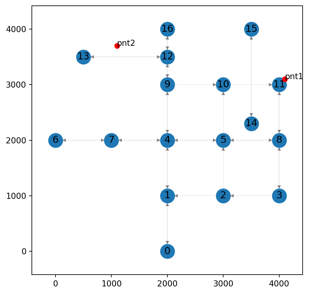
The simplest solution would be to calculate the route between the nodes nearest to each point. This is what we do next (Routing between nearest nodes). Later, we will explore a more accurate and complex solution, involving modification of the network itself (Custom location routing function).
Routing between nearest nodes
The basic network routing approach is to calculate the optimal route between existing nodes on the network (Basic routing function). The naive approach therefore may be to identify the nearest nodes to the locations of interest, and then to calculate the shortest path between the nodes.
Here is how we can identify the nearest nodes to pnt1 and pnt2, using the net2.nearest_node function (Nearest node):
node1 = net2.nearest_node(G, pnt1)
node1
(11, 141.4213562373095)node2 = net2.nearest_node(G, pnt2)
node2(13, 632.4555320336759)Now, the node IDs (node1[0] and node2[0]) can be passed to net2.route1 (Basic routing function) to find, for instance, the shortest route:
route = net2.route1(G, node1[0], node2[0], weight='length')
route
{'route': [11, 8, 5, 4, 9, 12, 13], 'weight': 6000.0}route = route['route']
route[11, 8, 5, 4, 9, 12, 13]Figure 9.2 displays the calculated route:
fig, ax = plt.subplots()
nx.draw(G, with_labels=True, pos=net2.pos(G), edge_color='grey', width=0.1, ax=ax)
nx.draw_networkx_edges(G, pos=net2.pos(G), edgelist=list(zip(route, route[1:])), edge_color='r', width=3)
plt.plot(pnt1.x, pnt1.y, 'ro')
plt.plot(pnt2.x, pnt2.y, 'ro')
ax.annotate('pnt1', [pnt1.x, pnt1.y], ha='left')
ax.annotate('pnt2', [pnt2.x, pnt2.y], ha='left')
plt.axis('on')
ax.set_aspect('equal')
ax.tick_params(left=True, bottom=True, labelleft=True, labelbottom=True);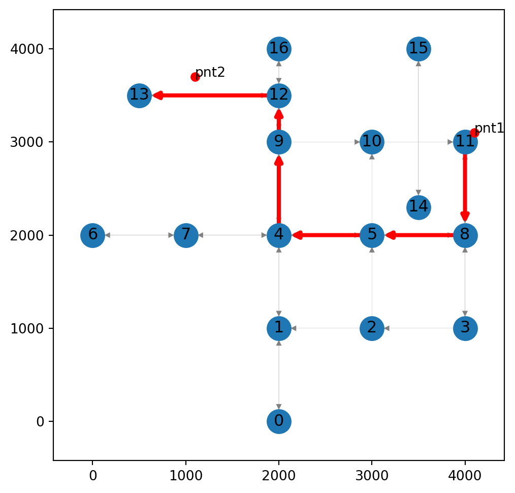
Adding new nodes—manual
The final segment in the calculated route 12→13, suggests an overesgtimation (Figure 9.2) of the traveled distance. To make the calculation more accurate, we are going to insert a new node into the road network, near pnt2.
Specifically, what we need to do is as follows:
- Add a new node
-1on the12↔︎13edges, at the point nearest topnt2, i.e.,(1100,3700) - Remove the
12→13edge, instead inserting new12→-1and-1→12edges - Remove the
13→12edge, instead inserting new13→-1and-1→13edges - Assign attributes to the four new edges
In this section, the changes are going to be made “manually”, in the sense that we are going to manually specify the indices of all the nodes involved. Later on, we are going to generalize the workflow (Adding new nodes—automatic) so that it can be defined as a function (Adding new nodes—function).
The point nearest to pnt2 on the network is pnt. This is where the new node -1 is going to be placed:
pnt = (1100, 3500)
pnt
(1100, 3500)Figure 9.3 shows the initial structure of the network, before any changes, along with the point where the new node is going to be placed:
fig, ax = plt.subplots()
nx.draw(G, with_labels=True, pos=net2.pos(G), edge_color='grey', width=0.1, ax=ax)
plt.plot(*pnt, 'ro')
plt.axis('on')
ax.tick_params(left=True, bottom=True, labelleft=True, labelbottom=True);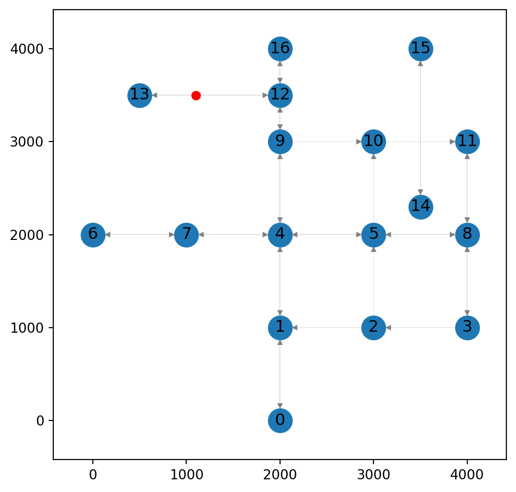
Now, let’s make the above-mentioned changes in the network. First, we add the new node, and the four new edges:
G.add_node(-1)
G.add_edge(12, -1)
G.add_edge(-1, 13)
G.add_edge(13, -1)
G.add_edge(-1, 12)
Next, we deal with the new node and edges’ attributes. The node 'geometry' attribute is according to pnt:
G.nodes[-1]['geometry'] = shapely.Point(pnt)Edges attributes are more complex:
'geometry'is a straight line, to or from the existing nodes12or13, to or from the new node-1'length'is according to the actual length of the new'geometry''time'is proportional to the edge length out of the total original length
Here is the calculation of these three attributes for the edge 12→-1:
# 'geometry' of the new edge
G.edges[12, -1]['geometry'] = shapely.LineString([
    G.nodes[12]['geometry'],
    G.nodes[-1]['geometry']
])
# 'length' of the new edge
G.edges[12, -1]['length'] = G.edges[12, -1]['geometry'].length# 'time' of the new edge
G.edges[12, -1]['time'] = G.edges[12, 13]['time'] * (G.edges[12, -1]['length'] / G.edges[12, 13]['length'])The calculated attributes are shown below:
G.edges[12, -1]{'geometry': <LINESTRING (2000 3500, 1100 3500)>,
'length': 900.0,
'time': 64.8}These calculations need to be repeated for the remaining three edges -1→12, 13→-1, and -1→13 (we won’t show the code here, to save space).
Finally, we can remove the “old” 12→13 and 13→12 edges:
G.remove_edge(12,13)
G.remove_edge(13,12)
Figure 9.4 shows the modified network:
fig, ax = plt.subplots()
nx.draw(G, with_labels=True, pos=net2.pos(G), edge_color='grey', width=0.1, ax=ax)
plt.plot(pnt2.x, pnt2.y, 'ro')
plt.axis('on')
ax.tick_params(left=True, bottom=True, labelleft=True, labelbottom=True);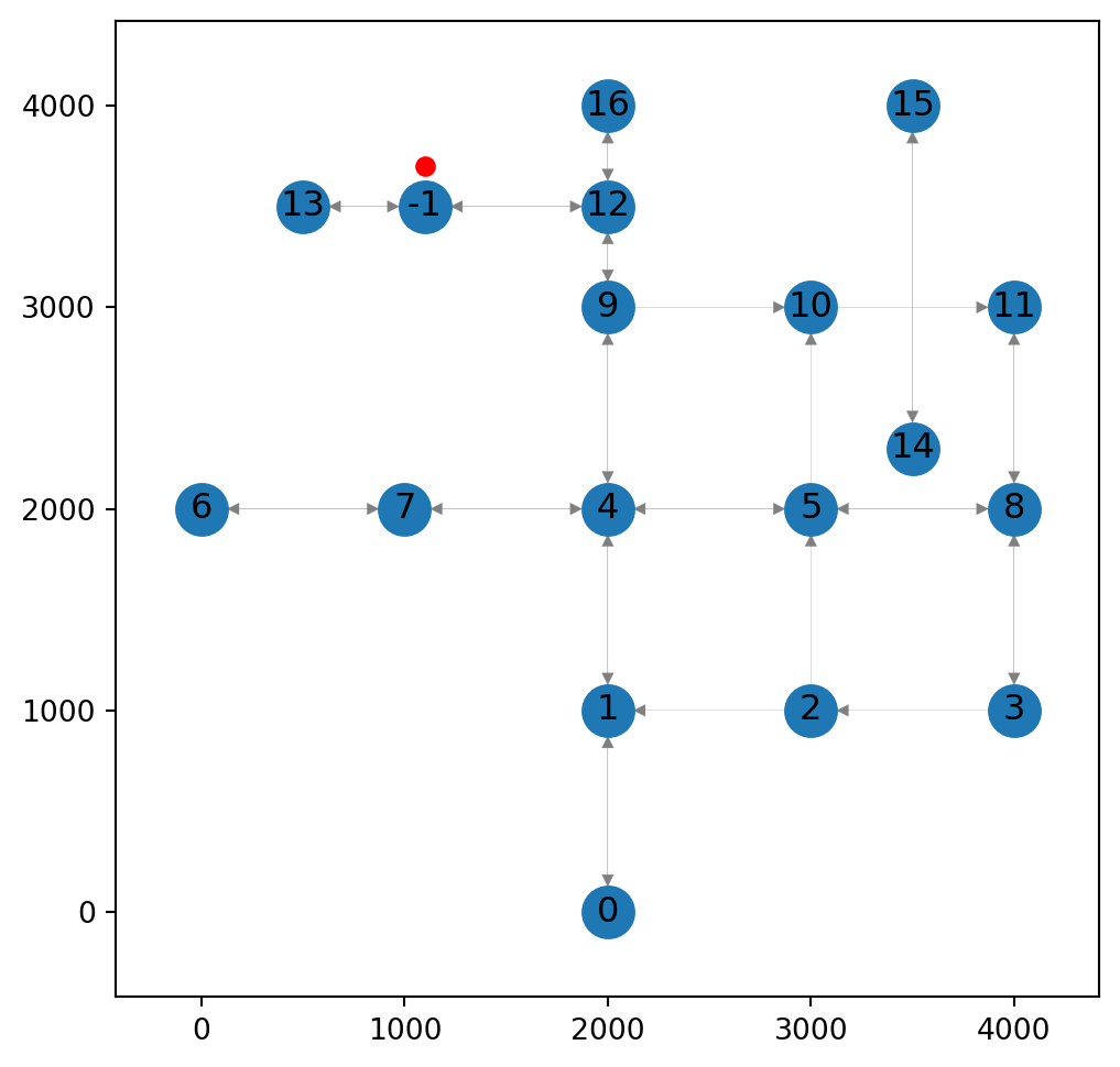
-1 and splitting the underlying edge into two “parts”
In the next section, we are going to make the network modification automatically, in a way that can be fitted into a function.
Before moving on, let’s re-load the original network:
G = nx.read_graphml('output/roads2.xml')
G = net2.prepare(G)
G
<networkx.classes.digraph.DiGraph at 0x737389647ec0>Adding new nodes—automatic
Overview
In this section, we are going to automate the procedure of inserting a new node into the network, placed on an existing edge, while “splitting” that edge. That is, we will write generalized code where, given the coordinates of a target point and the existing network, the new modified network is calculated and returned.
Suppose that we want to connect pnt2 to the network:
pnt2
The workflow is as follows:
- Detecting the nearest edge to
pnt2 - Locating the nearest point to
pnt2on that edge - Splitting the edge geometry into two parts
- Adding two new edges with those geometries, and calculating their other attributes
- Adding a new node at the splitting point
- Deleting the original edge
Finding nearest point
The first step is detecting the nearest edge. We do it using our net2.nearest_edge function:
nearest_edge = net2.nearest_edge(G, pnt2)
nearest_edge
((12, 13), 200.0)Given the edge ID e:
e = nearest_edge[0]
e
(12, 13)We can extract its properties from the network G:
G.edges[e]{'geometry': <LINESTRING (2000 3500, 500 3500)>,
'length': 1500.0,
'speed': 50,
'time': 108.0}Next we locate the point on the edge nearest to pnt2, using shapely.ops.nearest_points (Nearest point on line):
pnt_on_line = shapely.ops.nearest_points(G.edges[e]['geometry'], shapely.Point(pnt2))
pnt_on_line
(<POINT (1100 3500)>, <POINT (1100 3700)>)The function returns both the nearest point and the input point. We need just the former, naming it pnt_on_line:
pnt_on_line = pnt_on_line[0]
print(pnt_on_line)
POINT (1100 3500)Figure 9.5 shows the edge geometry, and the point on it which we calculated in the previous section:
shapely.GeometryCollection([G.edges[e]['geometry'], pnt_on_line])
The detected nearest point (Figure 9.5) is going to be a new node. The edge geometry is going to be split into two geometries of the two new edges.
Splitting the edge
The nearest point we found is passed to shapely.ops.split to split the line geometry into two parts. The parts are returned as a GeometryCollection:
lines = shapely.ops.split(G.edges[e]['geometry'], pnt_on_line)
print(lines)
GEOMETRYCOLLECTION (LINESTRING (2000 3500, 1100 3500), LINESTRING (1100 3500, 500 3500))Next, we extract the two line geometries into two separate objects, line1 and line2. However, we need to know which line “belongs” to each of the nodes on both sides of the original edge (G.nodes[e[0]] and G.nodes[e[1]]). Therefore, we first choose the line that intersects the first node and assign it to line1, and then choose the line which intersects with the second node, and assign it to line2:
p = G.nodes[e[0]]['geometry']
line1 = filter(p.intersects, lines.geoms)
line1 = list(line1)[0]
print(line1)
LINESTRING (2000 3500, 1100 3500)p = G.nodes[e[1]]['geometry']
line2 = filter(p.intersects, lines.geoms)
line2 = list(line2)[0]
print(line2)LINESTRING (1100 3500, 500 3500)
Note
filter is a built-in Python function that accepts a function and a sequence. The output is an iterator, which yields the filtered elements, i.e., those elements where the function returns True. In the above example, filter is applied on the function p.intersects and the sequence lines.geoms. As a result, filter returns the subset of lines geometries which intersect with p.
Now we can add the new node. We will choose an ID that is smaller than the minumum ID value, ensuring that there is no existing node with the same ID:
node_id = min(list(G.nodes))-1
node_id-1Now we add the node, at the pnt_on_line location:
G.add_node(node_id, geometry=pnt_on_line)We also have to add the two new edges. Note that:
- the 1st edge goes from the node
e[0]to the new nodenode_id, with the geometryline1 - the 2nd edge goes from the new node
node_idto the nodee[1], with the geometryline2
Therefore:
G.add_edge(e[0], node_id, geometry=line1, length=line1.length)
G.add_edge(node_id, e[1], geometry=line2, length=line2.length)
At this stage, we have a new node (-1) and the two new edges (12→-1 and -1→13) (Figure 9.6):
pnt2
nx.draw(G, with_labels=True, pos=net2.pos(G), connectionstyle='arc3,rad=0.2')
plt.plot(pnt2.x, pnt2.y, 'ro');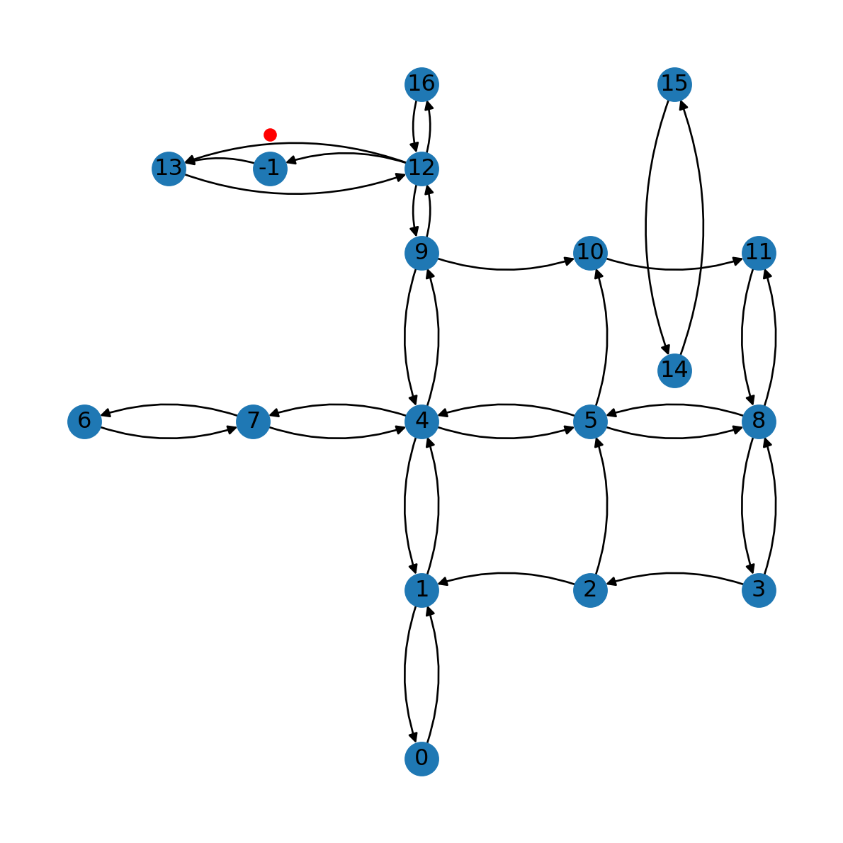
Now we can remove the original node:
G.remove_edge(*e)Here is the modified network (Figure 9.7):
nx.draw(G, with_labels=True, pos=net2.pos(G), connectionstyle='arc3,rad=0.2')
plt.plot(pnt2.x, pnt2.y, 'ro');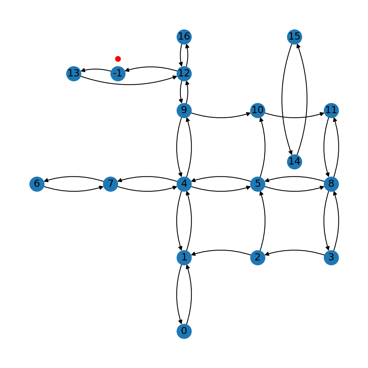
Assuming that there is a parallel edge in the opposite direction—which in this example there is—we need to repeat the prodedure to split it as well. First, we identify the edge, by reversing the node IDs:
e = (e[1], e[0])
e
(13, 12)Here is the opposite edge which we are going to modify right now:
G.edges[e]{'geometry': <LINESTRING (2000 3500, 500 3500)>,
'length': 1500.0,
'speed': 50,
'time': 108.0}First, we split the line into geometries line1 and line2, using the same code as above (Splitting the edge):
pnt_on_line = shapely.ops.nearest_points(G.edges[e]['geometry'], shapely.Point(pnt2))
pnt_on_line = pnt_on_line[0]
lines = shapely.ops.split(G.edges[e]['geometry'], pnt_on_line)
p = G.nodes[e[0]]['geometry']
line1 = filter(p.intersects, lines.geoms)
line1 = list(line1)[0]
p = G.nodes[e[1]]['geometry']
line2 = filter(p.intersects, lines.geoms)
line2 = list(line2)[0]
line1, line2
(<LINESTRING (1100 3500, 500 3500)>, <LINESTRING (2000 3500, 1100 3500)>)Then, we add the new edges and remove the old one:
G.add_edge(e[0], node_id, geometry=line1, length=line1.length)
G.add_edge(node_id, e[1], geometry=line2, length=line2.length)
G.remove_edge(*e)
The result is shown in Figure 9.8:
nx.draw(G, with_labels=True, pos=net2.pos(G), connectionstyle='arc3,rad=0.2')
plt.plot(pnt2.x, pnt2.y, 'ro');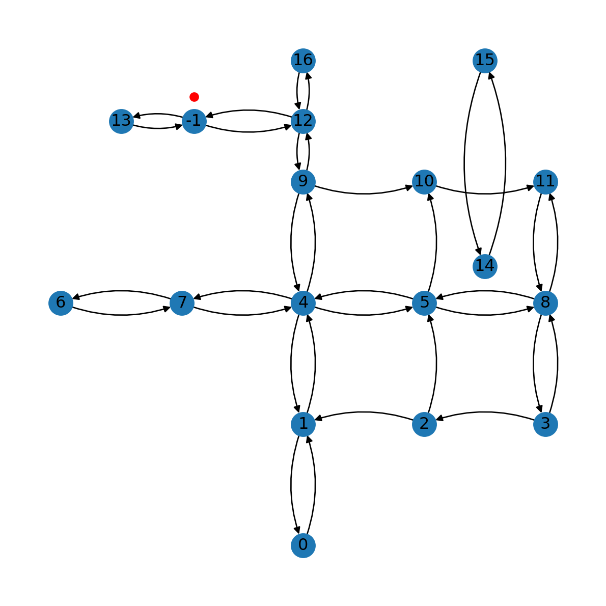
Adding new nodes—function
First example
To apply the workflow shown in Adding new nodes—automatic more systematically, we are going to use a function named net2.add_node. The function accepts a network G, and a point pnt, and returns:
- a (possibly modified) network,
- the nearest node to
pnton the (possibly modified) networkG, and - the distance from
pntto the nearest node
The function goes through one of the following scenarios:
- If
pntis exactly on an existing node → return unchangedG, that node, and distance0 - If nearest point to
pntonGis an existing node → return unchangedG, that node, and distance to the node - If nearest point to
pntonGis not existing node → insert new node and return modifiedG, the new node, and distance to new node
Note
The code of net2.add_node uses the principles shown above, but also expands it to deal with several edge cases. Going over the entire source code of net2.add_node is beyond the scope of this book.
In Adding new nodes—automatic we’ve actually seen an example of scenario (3). Let’s repeat it using the net2.add_node function.
First, we re-import the network data to start from the original unmodified network:
G = nx.read_graphml('output/roads2.xml')
G = net2.prepare(G)
G
<networkx.classes.digraph.DiGraph at 0x73738a0c9e20>And now we apply the net2.add_node function to add the new node at the location nearest to pnt2. Note that the function returns the modified network, the new node ID (-1), and the distance from pnt2 to the new node (200.0 \(m\)):
result = net2.add_node(G, pnt2)
result
(<networkx.classes.digraph.DiGraph at 0x7373898ed880>, -1, 200.0)Let’s extract just the network:
G = result[0]
G
<networkx.classes.digraph.DiGraph at 0x7373898ed880>The result, which is the same as Figure 9.8, is shown in Figure 9.9:
fig, ax = plt.subplots()
nx.draw(G, with_labels=True, pos=net2.pos(G), ax=ax)
plt.plot(pnt2.x, pnt2.y, 'ro');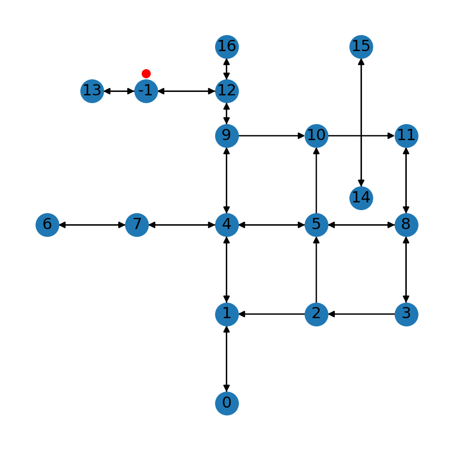
-1) inserted into the roads network using the net2.add_node function
Point on existing node
Here is an example of scenario 1, when the queried point on the network is already an existing node:
pnt = shapely.Point(4000, 3000)
x = net2.add_node(G, pnt)
x
(<networkx.classes.digraph.DiGraph at 0x737389f030e0>, 11, 0.0)In such case, as shown in the above output, the node itself (11) is returned along with a distance of 0.
Figure 9.10 illustrates scenario 1:
fig, ax = plt.subplots()
nx.draw(x[0], with_labels=True, pos=net2.pos(x[0]), ax=ax)
plt.plot(pnt.x, pnt.y, 'ro')
plt.axis('on')
ax.tick_params(left=True, bottom=True, labelleft=True, labelbottom=True);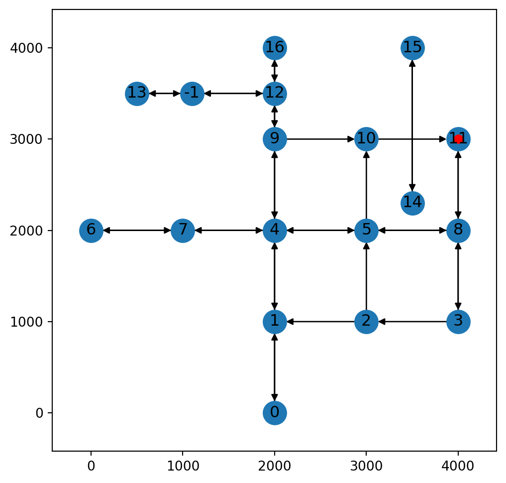
net2.add_node function, where the point of interest is exactly on an existing node
Point nearest to an existing node
Here is an example of scenario 2, when the nearest point on the network is already an existing node:
pnt = shapely.Point(4200, 3200)
x = net2.add_node(G, pnt)
x
(<networkx.classes.digraph.DiGraph at 0x7373898899d0>, 11, 282.842712474619)In this case, we can see that the returned node ID is 11, which is the ID of the nearest existing node. Figure 9.11 illustrates scenario 2:
fig, ax = plt.subplots()
nx.draw(x[0], with_labels=True, pos=net2.pos(x[0]), ax=ax)
plt.plot(pnt.x, pnt.y, 'ro')
plt.axis('on')
ax.tick_params(left=True, bottom=True, labelleft=True, labelbottom=True);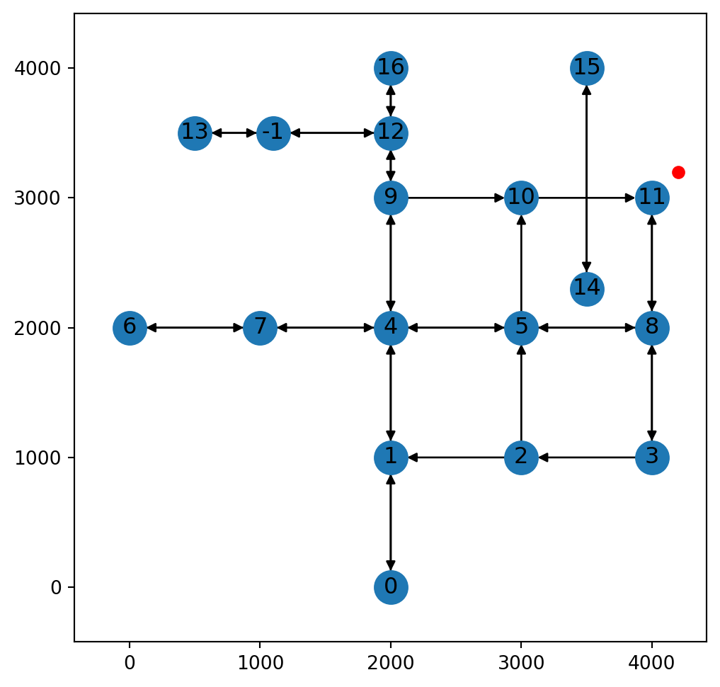
net2.add_node function, where the nearest point on the network is an existing node
Inserting new node (two-way)
Here is an the 1st example of scenario 3, where a new node is being added into a two-way road segment:
pnt = shapely.Point(4300, 2600)
x = net2.add_node(G, pnt)
x
(<networkx.classes.digraph.DiGraph at 0x7373895e6ed0>, -2, 300.0)Figure 9.12 illustrates scenario 3, where a where a new node is inserted into a two-way edge:
fig, ax = plt.subplots()
nx.draw(x[0], with_labels=True, pos=net2.pos(x[0]), ax=ax)
plt.plot(pnt.x, pnt.y, 'ro')
plt.axis('on')
ax.tick_params(left=True, bottom=True, labelleft=True, labelbottom=True);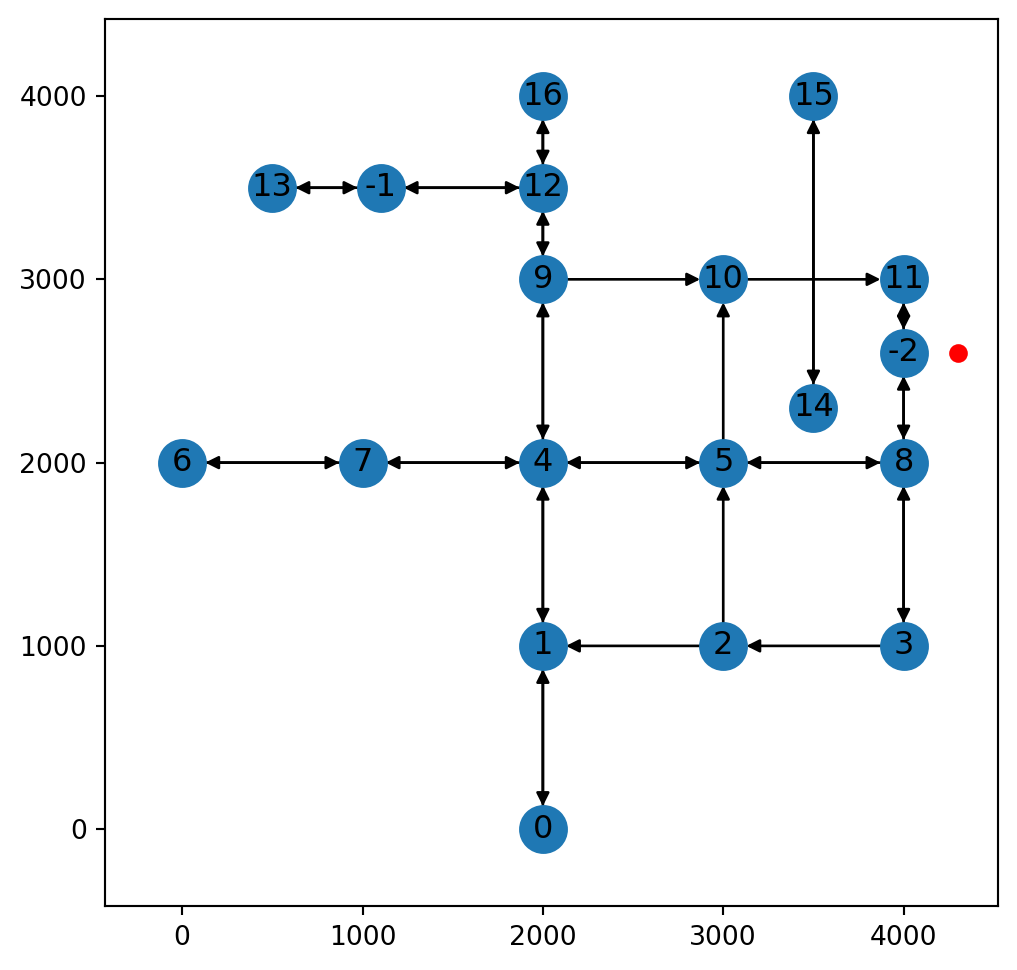
net2.add_node function, where a new node is inserted into a two-way edge
Inserting new node (one-way)
Here is the 2nd example of scenario 3, where a new node is being added into a one-way road segment:
pnt = shapely.Point(3600, 700)
x = net2.add_node(G, pnt)
x
(<networkx.classes.digraph.DiGraph at 0x7373894ac380>, -2, 300.0)Figure 9.12 illustrates scenario 3, where a where a new node is inserted into a one-way edge:
fig, ax = plt.subplots()
nx.draw(x[0], with_labels=True, pos=net2.pos(x[0]), ax=ax)
plt.plot(pnt.x, pnt.y, 'ro')
plt.axis('on')
ax.tick_params(left=True, bottom=True, labelleft=True, labelbottom=True);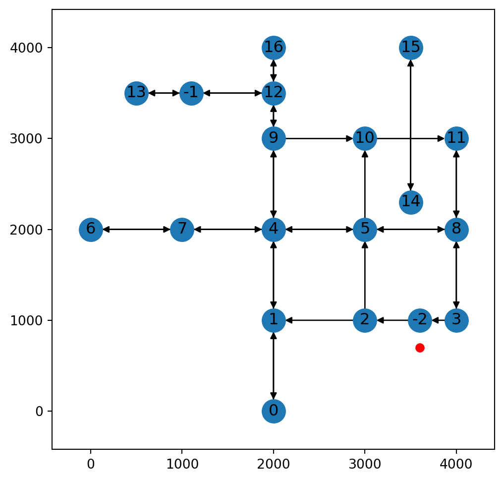
net2.add_node function, where a new node is inserted into a one-way edge
Custom location routing function
Now that we defined the net2.add_node function (Adding new nodes—function), we can warp it into a routing function, which calculates an optimal route while also inserting new nodes into the network where necessary.
To demonstrate, let’s re-import the roads network:
G = nx.read_graphml('output/roads2.xml')
G = net2.prepare(G)
G
<networkx.classes.digraph.DiGraph at 0x7373896e5e20>Suppose that we have two point locations, pnt1 and pnt2:
pnt1 = shapely.Point(4100, 3100)
pnt2 = shapely.Point(1100, 3700)
The function we define for routing while adding new nodes is called net2.route2. Here is its source code:
def route2(network, start, end, weight):
    network, node_start, dist_start = add_node(network, start)
    network, node_end, dist_end = add_node(network, end)
    try:
        route = nx.shortest_path(network, node_start, node_end, weight)
        weight_sum = nx.path_weight(network, route, weight=weight)
    except:
        route = np.nan
        weight_sum = np.nan
    return {
            'route': route,
            'weight': weight_sum,
            'dist_start': dist_start,
            'dist_end': dist_end,
            'network': network
        }
The source code of net2.route2 is basically an expanded version of net2.route2 (Basic routing function). The net2.route2 adds new nodes using net2.add_node. It also returns the 'dist_start' and 'dist_end' attributes, which express the distance from the input points to the (possibly new) node on the network.
Let’s apply the net2.route2 function to find the shortest route from pnt1 to pnt2:
x = net2.route2(G, pnt1, pnt2, 'length')
x
{'route': [11, 8, 5, 4, 9, 12, -1],
'weight': 5400.0,
'dist_start': 141.4213562373095,
'dist_end': 200.0,
'network': <networkx.classes.digraph.DiGraph at 0x7373896229f0>}Figure 9.14 shows the calculated route along with the modified network:
fig, ax = plt.subplots()
nx.draw(x['network'], with_labels=True, pos=net2.pos(x['network']), edge_color='grey', width=0.1, ax=ax)
nx.draw_networkx_edges(G, pos=net2.pos(x['network']), edgelist=list(zip(x['route'], x['route'][1:])), edge_color='r', width=3)
plt.plot(pnt1.x, pnt1.y, 'ro')
plt.plot(pnt2.x, pnt2.y, 'ro')
ax.annotate('pnt1', [pnt1.x, pnt1.y], ha='left')
ax.annotate('pnt2', [pnt2.x, pnt2.y], ha='left')
plt.axis('on')
ax.tick_params(left=True, bottom=True, labelleft=True, labelbottom=True);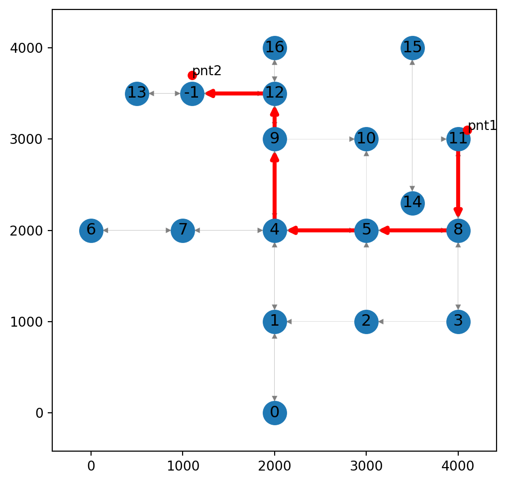
(4200, 1500) to (1100, 400) while inserting new nodes into the network, using the net2.route2 function
Exercises
Exercise 08-01
- Using the railway network from Exercise 06-02, calculate the fastest route from Netanya to Beer-Sheva
- Plot the modified network with the calculated route
- Calculate and print the travel times from Haifa to Lod, and then from Netanya to Lod (which should be smaller)
Exercise 08-02
- Use the following code section to prepare the road network
Gand a list of 250 random points covering the networks’ extentpoints; The network and the points are shown in Figure 19.17.
import numpy as np
import shapely
import networkx as nx
import net2
# Prepare road network
G = nx.read_graphml('output/roads2.xml')
G = net2.prepare(G)
# Prepare random points
edges = net2.edges_to_gdf(G)
bounds = edges.buffer(250).total_bounds
xmin, ymin, xmax, ymax = bounds
points = []
while len(points) < 300:
    random_point = shapely.Point([np.random.uniform(xmin, xmax), np.random.uniform(ymin, ymax)])
points.append(random_point)- Use the
net2.add_nodefunction on each of the 250 points, to calculate location of the new/existing nearest nodes to each of the points - Plot the 250 points, their associated nodes on the network, and line segments between each pair (Figure 19.18)
Exercise 08-03
- Use the principles from this chapter to modify the road network in such as way that there is a (10,11) (14,15)